Least Squares Approximations

Section 26 Least Squares Approximations

Focus Questions

By the end of this section, you should be able to give precise and thorough answers to the questions listed below. You may want to keep these questions in mind to focus your thoughts as you complete the section.

How, in general, can we find a least squares approximation to a system $A x = b ?$
If the columns of $A$ are linearly independent, how can we find a least squares approximation to $A x = b$ using just matrix operations?
Why are these approximations called “least squares” approximations?

🔗

Subsection Application: Fitting Functions to Data

🔗

Data is all around us. Data is collected on almost everything and it is important to be able to use data to make predictions. However, data is rarely well-behaved and so we generally need to use approximation techniques to estimate from the data. One technique for this is least squares approximations. As we will see, we can use linear algebra to fit a variety of different types of curves to data.

🔗

Subsection Introduction

🔗

In this section our focus is on fitting linear and polynomial functions to data sets.

🔗

Preview Activity 26.1.

NBC was awarded the U.S. television broadcast rights to the 2016 and 2020 summer Olympic games. Table 26.1 lists the amounts paid (in millions of dollars) by NBC sports for the 2008 through 2012 summer Olympics plus the recently concluded bidding for the 2016 and 2020 Olympics, where year 0 is the year 2008. (We will assume a simple model here, ignoring variations such as value of money due to inflation, viewership data which might affect NBC's expected revenue, etc.) Figure 26.2 shows a plot of the data. Our goal in this activity is to find a linear function $f$ defined by $f (x) = a_{0} + a_{1} x$ that fits the data well.

Table 26.1. Olympics television broadcast rights.

Year	Amount
0	894
4	1180
8	1226
12	1418

If the data were actually linear, then the data would satisfy the system

\begin{aligned} a_{0} & + & 0 a_{1} & = & 894 \\ a_{0} & + & 4 a_{1} & = & 1180 \\ a_{0} & + & 8 a_{1} & = & 1226 \\ a_{0} & + & 12 a_{1} & = & 1418 & . \end{aligned}

The vector form of this equation is

a_{0} [1 1 1 1]^{T} + a_{1} [0 4 8 12]^{T} = [894 1180 1226 1418]^{T} .

This equation does not have a solution, so we seek the best approximation to a solution we can find. That is, we want to find $a_{0}$ and $a_{1}$ so that the line $f (x) = a_{0} + a_{1} x$ provides a best fit to the data.

Letting $v_{1} = [1 1 1 1]^{T}$ and $v_{2} = [0 4 8 12]^{T},$ and $b = [894 1180 1226 1418]^{T},$ our vector equation becomes

a_{0} v_{1} + a_{1} v_{2} = b .

To make a best fit, we will minimize the square of the distance between $b$ and a vector of the form $a_{0} v_{1} + a_{1} v_{2} .$ That is, minimize

\begin{matrix} (26.1) & | | b - (a_{0} v_{1} + a_{1} v_{2}) | |^{2} . \end{matrix}

Rephrasing this in terms of projections, we are looking for the vector in $W = Span {v_{1}, v_{2}}$ that is closest to $b .$ In other words, the values of $a_{0}$ and $a_{1}$ will occur as the weights when we write ${proj}_{W} b$ as a linear combination of $v_{1}$ and $v_{2} .$ The one wrinkle in this problem is that we need an orthogonal basis for $W$ to find this projection. Use appropriate technology throughout this activity.

🔗

(a)

Find an orthogonal basis $B = {w_{1}, w_{2}}$ for $W .$

🔗

(b)

Use the basis $B$ to find $y = {proj}_{W} b$ as illustrated in Figure 26.3.

🔗

(c)

Find the values of $a_{0}$ and $a_{1}$ that give our best fit line by writing $y$ as a linear combination of $v_{1}$ and $v_{2} .$

🔗

(d)

Draw a picture of your line from the previous part on the axes with the data set. How well do you think your line approximates the data? Explain.

🔗

Subsection Least Squares Approximations

🔗

In Section 25 we saw that the projection of a vector

v

R^{n}

onto a subspace

W

R^{n}

is the best approximation to

v

of all the vectors in

W .

In fact, if

v = [v_{1} v_{2} \dots v_{n}]^{T}

and

{proj}_{W} v = [w_{1} w_{2} w_{3} \dots w_{m}]^{T},

then the error in approximating

v

w

is given by

| | v - {proj}_{W} v | |^{2} = \sum_{i = 1}^{m} (v_{i} - w_{i})^{2} .

🔗

In the context of Preview Activity 26.1, we projected the vector

b

onto the span of the vectors

v_{1} = [1 1 1 1]^{T}

and

v_{2} = [0 4 8 12]^{T} .

The projection minimizes the distance between the vectors in

W

and the vector

b

(as shown in Figure 26.3), and also produces a line which minimizes the sums of the squares of the vertical distances from the line to the data set as illustrated in Figure 26.4 with the olympics data. This is why these approximations are called least squares approximations.

🔗
Figure 26.4. Least squares linear approximation

🔗

While we can always solve least squares problems using projections, we can often avoid having to create an orthogonal basis when fitting functions to data. We work in a more general setting, showing how to fit a polynomial of degree

n

to a set of data points. Our goal is to fit a polynomial

p (x) = a_{0} + a_{1} x + a_{2} x^{2} + \dots + a_{n} x^{n}

of degree

n

m

data points

(x_{1}, y_{1}),

(x_{2}, y_{2}),

\dots,

(x_{m}, y_{m}),

no two of which have the same

x

coordinate. In the unlikely event that the polynomial

p (x)

actually passes through the

m

points, then we would have the

m

equations

\begin{aligned} (26.2) & y_{1} & = & a_{0} & + & a_{1} x_{1} & + & a_{2} x_{1}^{2} & + & \dots & + & a_{n - 1} x_{1}^{n - 1} & + & a_{n} x_{1}^{n} \\ (26.3) & y_{2} & = & a_{0} & + & a_{1} x_{2} & + & a_{2} x_{2}^{2} & + & \dots & + & a_{n - 1} x_{2}^{n - 1} & + & a_{n} x_{2}^{n} \\ (26.4) & y_{3} & = & a_{0} & + & a_{1} x_{3} & + & a_{2} x_{3}^{2} & + & \dots & + & a_{n - 1} x_{3}^{n - 1} & + & a_{n} x_{3}^{n} \\ (26.5) & ⋮ \\ (26.6) & y_{m} & = & a_{0} & + & a_{1} x_{m} & + & a_{2} x_{m}^{2} & + & \dots & + & a_{n - 1} x_{m}^{n - 1} & + & a_{n} x_{m}^{n} \end{aligned}

🔗

in the

n + 1

unknowns

a_{0},

a_{1},

\dots,

a_{n - 1},

and

a_{n} .

🔗

The

m

data points are known in this situation and the coefficients

a_{0},

a_{1},

\dots,

a_{n}

are the unknowns. To write the system in matrix-vector form, the coefficient matrix

M

M = [\begin{array}{cccccc} 1 & x_{1} & x_{1}^{2} & \dots & x_{1}^{n - 1} & x_{1}^{n} \\ 1 & x_{2} & x_{2}^{2} & \dots & x_{2}^{n - 1} & x_{2}^{n} \\ 1 & x_{3} & x_{3}^{2} & \dots & x_{3}^{n - 1} & x_{3}^{n} \\ ⋮ & ⋮ & ⋮ & \dots & ⋮ & ⋮ \\ 1 & x_{m} & x_{m}^{2} & \dots & x_{m}^{n - 1} & x_{m}^{n} \end{array}],

🔗

while the vectors

a

and

y

are

a = [\begin{matrix} a_{0} \\ a_{1} \\ a_{2} \\ ⋮ \\ a_{n - 1} \\ a_{n} \end{matrix}] and y = [\begin{matrix} y_{1} \\ y_{2} \\ y_{3} \\ ⋮ \\ y_{m - 1} \\ y_{m} \end{matrix}] .

🔗

Letting

y = [y_{1} y_{2} \dots y_{m}]^{T}

and

v_{i} = [x_{1}^{i - 1} x_{2}^{i - 1} \dots x_{m}^{i - 1}]^{T}

for

1 \leq i \leq n + 1,

the vector form of the system is

y = a_{0} v_{1} + a_{1} v_{2} + \dots + a_{n} v_{n + 1} .

🔗

Of course, it is unlikely that the

m

data points already lie on a polynomial of degree

n,

so the system will usually have no solution. So instead of attempting to find coefficients

a_{0},

a_{1},

\dots,

a_{n}

that give a solution to this system, which may be impossible, we instead look for a vector that is ``close" to a solution. As we have seen, the vector

{proj}_{W} y,

where

W

is the span of the columns of

M,

minimizes the sum of the squares of the differences of the components. That is, our desired approximation to a solution to

M x = y

is the projection of

y

onto

Col M .

Now

{proj}_{W} y

is a linear combination of the columns of

M,

{proj}_{W} y = M a^{*}

for some vector

a^{*} .

This vector

a^{*}

then minimizes

| | {proj}_{⊥ W} y | | = | | y - M a | | .

That is, if we let

(M a)^{T} = [b_{1} b_{2} b_{3} \dots b_{m}],

we are minimizing

\begin{matrix} (26.7) & | | y - M a | |^{2} = (y_{1} - b_{1})^{2} + (t_{2} - b_{2})^{2} + \dots + (y_{m} - b_{m})^{2} . \end{matrix}

🔗

The expression

| | y - M a | |^{2}

measures the error in our approximation.

🔗

The question we want to answer is how we can find the vector

a^{*}

that minimizes

| | y - M a | |

in a way that is more convenient than computing a projection. We answer this question in a general setting in the next activity.

🔗

Activity 26.2.

Let $A$ be an $m \times n$ matrix and let $b$ be in $R^{m} .$ Let $W = Col A .$ Then ${proj}_{W} b$ is in $Col A,$ so let $x^{*}$ be in $R^{n}$ such that $A x^{*} = {proj}_{W} b .$

🔗

(a)

Explain why $b - A x^{*}$ is orthogonal to every vector of the form $A x,$ for any $x$ in $R^{n} .$ That is, $b - A x^{*}$ is orthogonal to $Col A .$

🔗

(b)

Let $a_{i}$ be the $i$ th column of $A .$ Explain why $a_{i} \cdot (b - A x^{*}) = 0 .$ From this, explain why $A^{T} (b - A x^{*}) = 0 .$

🔗

(c)

From the previous part, show that $x^{*}$ satisfies the equation

A^{T} A x^{*} = A^{T} b .

🔗

The result of Activity 26.2 is that we can now do least squares polynomial approximations with just matrix operations. We summarize this in the following theorem.

🔗

Theorem 26.5.

The least squares solutions to the system $A x = b$ are the solutions to the corresponding system

\begin{matrix} (26.8) & A^{T} A x = A^{T} b . \end{matrix}

🔗

The equations in the system (26.8) are called the normal equations for

A x = b .

To illustrate, with the Olympics data, our data points are

(0, 894),

(4, 1180),

(8, 1226),

(12, 1418)

with

y = [894 1180 1226 1418]^{T} .

M = [\begin{array}{cc} 1 & 0 \\ 1 & 4 \\ 1 & 8 \\ 1 & 12 \end{array}] .

Notice that

M^{T} M

is invertible, to find the degree 1 approximation to the data, technology shows that

a^{*} = {(M^{T} M)}^{- 1} M^{T} y = [\frac{4684}{5} \frac{809}{20}]

🔗

just as in Preview Activity 26.1.

🔗

Activity 26.3.

Now use the least squares method to find the best polynomial approximations (in the least squares sense) of degrees 2 and 3 for the Olympics data set in Table 26.1. Which polynomial seems to give the “best” fit? Explain why. Include a discussion of the errors in your approximations. Use your “best” least squares approximation to estimate how much NBC might pay for the television rights to the 2024 Olympic games. Use technology as appropriate.

🔗

The solution with our Olympics data gave us the situation where

M^{T} M

was invertible. This corresponded to a unique least squares solution

{(M^{T} M)}^{- 1} M^{T} y .

It is reasonable to ask when this happens in general. To conclude this section, we will demonstrate that if the columns of a matrix

A

are linearly independent, then

A^{T} A

🔗

Theorem 26.6.

If the columns of $A$ are linearly independent, then the least squares solution $x^{*}$ to the system $A x = b$ is

x^{*} = {(A^{T} A)}^{- 1} A^{T} b .

🔗

If the columns of

A

are linearly dependent, we can still solve the normal equations, but will obtain more than one solution. In a later section we will see that we can also use a pseudoinverse in these situations.

🔗

Subsection Examples

🔗

What follows are worked examples that use the concepts from this section.

🔗

Example 26.7.

According to the Centers for Disease Control and Prevention ⁴⁵, the average length of a male infant (in centimeters) in the US as it ages (with time in months from 1.5 to 8.5) is given in Table 26.8.

Table 26.8. Average lengths of male infants

Age (months)	1.5	2.5	3.5	4.5	5.5	6.5	7.5	8.5
Average Length (cm)	56.6	59.6	62.1	64.2	66.1	67.9	69.5	70.9

In this problem we will find the line and the quadratic of best fit in the least squares sense to this data. We treat age in months as the independent variable and length in centimeters as the dependent variable.

🔗

(a)

Find a line that is the best fit to the data in the least squares sense. Draw a picture of your least squares solution against a scatterplot of the data.

Solution.

We assume that a line of the form $f (x) = a_{1} x + a_{0}$ contains all of the data points. The first data point would satisfy $1.5 a_{1} + a_{0} = 56.6,$ the second $2.5 a_{1} + a_{0} = 59.6,$ and so on, giving us the linear system

\begin{aligned} 3 1.5 a_{1} & + & a_{0} & = 56.6 \\ 2.5 a_{1} & + & a_{0} & = 59.6 \\ 3.5 a_{1} & + & a_{0} & = 62.1 \\ 4.5 a_{1} & + & a_{0} & = 64.2 \\ 5.5 a_{1} & + & a_{0} & = 66.1 \\ 6.5 a_{1} & + & a_{0} & = 67.9 \\ 7.5 a_{1} & + & a_{0} & = 69.5 \\ 8.5 a_{1} & + & a_{0} & = 70.9 . \end{aligned}

Letting

A = [\begin{array}{cc} 1.5 & 1 \\ 2.5 & 1 \\ 3.5 & 1 \\ 4.5 & 1 \\ 5.5 & 1 \\ 6.5 & 1 \\ 7.5 & 1 \\ 8.5 & 1 \end{array}], x = [\begin{matrix} a_{1} \\ a_{0} \end{matrix}], and b = [\begin{matrix} 56.6 \\ 59.6 \\ 62.1 \\ 64.2 \\ 66.1 \\ 67.9 \\ 69.5 \\ 70.9 \end{matrix}],

we can write this system in the matrix form $A x = b .$ Neither column of $A$ is a multiple of the other, so the columns of $A$ are linearly independent. The least squares solution $x^{*}$ to the system is then found by

x^{*} = {(A^{T} A)}^{- 1} A^{T} b .

Technology shows that (with entries rounded to 3 decimal places), ${(A^{T} A)}^{- 1} A^{T}$ is

[\begin{array}{rrrrcrrr} - 0.083 & - 0.060 & - 0.036 & - 0.012 & 0.012 & 0.036 & 0.060 & 0.083 \\ 0.542 & 0.423 & 0.304 & 0.185 & 0.065 & - 0.054 & - 0.173 & - 0.292 \end{array}],

and

x^{*} \approx [\begin{array}{cc} 2.011 \\ 54.559 \end{array}] .

So the least squares linear function to the data is $f (x) \approx 2.011 x + 54.559 .$ A graph of $f$ against the data points is shown at left in Figure 26.9.

Figure 26.9. Left: Least squares line. Right: Least squares quadratic.

🔗

(b)

Now find the least squares quadratic of the form $q (x) = a_{2} x^{2} + a_{1} x + a_{0}$ to the data. Draw a picture of your least squares solution against a scatterplot of the data.

Solution.

The first data point would satisfy $({1.5}^{2}) a_{2} + 1.5 a_{1} + a_{0} = 56.6,$ the second $(2.5)^{2} a_{2} + 2.5 a_{1} + a_{0} = 59.6,$ and so on, giving us the linear system

\begin{aligned} {1.5}^{2} a_{2} & + & 1.5 a_{1} & + & a_{0} & = 56.6 \\ {2.5}^{2} a_{2} & + & 2.5 a_{1} & + & a_{0} & = 59.6 \\ {3.5}^{2} a_{2} & + & 3.5 a_{1} & + & a_{0} & = 62.1 \\ {4.5}^{2} a_{2} & + & 4.5 a_{1} & + & a_{0} & = 64.2 \\ {5.5}^{2} a_{2} & + & 5.5 a_{1} & + & a_{0} & = 66.1 \\ {6.5}^{2} a_{2} & + & 6.5 a_{1} & + & a_{0} & = 67.9 \\ {7.5}^{2} a_{2} & + & 7.5 a_{1} & + & a_{0} & = 69.5 \\ {8.5}^{2} a_{2} & + & 8.5 a_{1} & + & a_{0} & = 70.9 . \end{aligned}

Letting

A = [\begin{array}{ccc} {1.5}^{2} & 1.5 & 1 \\ {2.5}^{2} & 2.5 & 1 \\ {3.5}^{2} & 3.5 & 1 \\ {4.5}^{2} & 4.5 & 1 \\ {5.5}^{2} & 5.5 & 1 \\ {6.5}^{2} & 6.5 & 1 \\ {7.5}^{2} & 7.5 & 1 \\ {8.5}^{2} & 8.5 & 1 \end{array}], x = [\begin{matrix} a_{2} \\ a_{1} \\ a_{0} \end{matrix}], and b = [\begin{matrix} 56.6 \\ 59.6 \\ 62.1 \\ 64.2 \\ 66.1 \\ 67.9 \\ 69.5 \\ 70.9 \end{matrix}],

we can write this system in the matrix form $A x = b .$ Technology shows that every column of the reduced row echelon form of $A$ contains a pivot, so the columns of $A$ are linearly independent. The least squares solution $x^{*}$ to the system is then found by

x^{*} = {(A^{T} A)}^{- 1} A^{T} b .

Technology shows that (with entries rounded to 3 decimal places) ${(A^{T} A)}^{- 1}$ is

[\begin{array}{rrrrrrrr} 0.042 & 0.006 & - 0.018 & - 0.030 & - 0.030 & - 0.018 & 0.006 & 0.042 \\ - 0.500 & - 0.119 & 0.143 & 0.286 & 0.310 & 0.214 & 0.000 & - 0.333 \\ 1.365 & 0.540 & - 0.049 & - 0.403 & - 0.522 & - 0.406 & - 0.055 & 0.531 \end{array}],

and

x^{*} \approx [\begin{array}{r} - 0.118 \\ 3.195 \\ 52.219 \end{array}] .

So the least squares quadratic function to the data is $q$ defined by $q (x) \approx - 0.118 x^{2} + 3.195 x + 52.219 .$ A graph of $q$ against the data points is shown at right in Figure 26.9.

🔗

Example 26.10.

Least squares solutions can be found through a QR factorization, as we explore in this example. Let $A$ be an $m \times n$ matrix with linearly independent columns and QR factorization $A = Q R .$ Suppose that $b$ is not in $Col A$ so that the system $A x = b$ is inconsistent. We know that the least squares solution $x^{*}$ to $A x = b$ is

\begin{matrix} (26.9) & x^{*} = {(A^{T} A)}^{- 1} A^{T} b . \end{matrix}

🔗

(a)

Replace $A$ by its QR factorization in (26.9) to show that

x^{*} = R^{- 1} Q^{T} b .

Hint.

Use the fact that $Q$ is orthogonal and $R$ is invertible.

Solution.

Replacing $A$ with $Q R$ and using the fact that $R$ is invertible and $Q$ is orthogonal to see that

\begin{aligned} x^{*} & = {(A^{T} A)}^{- 1} A^{T} b \\ = {((Q R)^{T} Q R)}^{- 1} (Q R)^{T} b \\ = (R^{T} Q^{T} Q R) R^{T} Q^{T} b \\ = {(R^{T} R)}^{- 1} R^{T} Q^{T} b \\ = R^{- 1} {(R^{T})}^{- 1} R^{T} Q^{T} b \\ = R^{- 1} Q^{T} b . \end{aligned}

So if $A = Q R$ is a QR factorization of $A,$ then the least squares solution to $A x = b$ is $R^{- 1} Q^{T} b .$

🔗

(b)

Consider the data set in Table 26.11, which shows the average life expectance in years in the US for selected years from 1950 to 2010.

Table 26.11. Life expectancy in the US

year	1950	1965	1980	1995	2010
age	68.14	70.21	73.70	75.98	78.49

(Data from macrotrends ⁴⁶.)

🔗

(i)

Use (26.9) to find the least squares linear fit to the data set.

Solution.

A linear fit to the data will be provided by the least squares solution to $A x = b,$ where

A = [\begin{array}{cc} 1 & 1950 \\ 1 & 1965 \\ 1 & 1980 \\ 1 & 1995 \\ 1 & 2010 \end{array}], x = [\begin{matrix} a \\ b \end{matrix}], and b = [\begin{matrix} 68.14 \\ 70.21 \\ 73.70 \\ 75.98 \\ 78.49 \end{matrix}] .

Technology shows that

{(A^{T} A)}^{- 1} A^{T} b \approx [- 276.1000 0.1765]^{T} .

🔗

(ii)

Use appropriate technology to find the QR factorization of an appropriate matrix $A,$ and use the QR decomposition to find the least squares linear fit to the data. Compare to what you found in part i.

Solution.

Technology shows that $A = Q R,$ where

Q = [\begin{array}{cr} \frac{1}{\sqrt{5}} & - \frac{2}{\sqrt{10}} \\ \frac{1}{\sqrt{5}} & - \frac{1}{\sqrt{10}} \\ \frac{1}{\sqrt{5}} & 0 \\ \frac{1}{\sqrt{5}} & \frac{1}{\sqrt{10}} \\ \frac{1}{\sqrt{5}} & \frac{2}{\sqrt{10}} \end{array}] and R = [\begin{array}{cc} \sqrt{5} & 1980 \sqrt{5} \\ 0 & 15 \sqrt{10} \end{array}] .

Then we have that

R^{- 1} Q^{T} b \approx [- 276.1000 0.1765]^{T},

just as in part i.

🔗

Subsection Summary

A least squares approximation to $A x = b$ is found by orthogonally projecting $b$ onto $Col A .$
If the columns of $A$ are linearly independent, then the least squares approximation to $A x = b$ is ${(A^{T} A)}^{- 1} A^{T} b .$
The least squares solution to $A x = b,$ where $A x = [y_{1} y_{2} \dots y_{m}]$ and $b = [b_{1} b_{2} \dots b_{m}]^{T},$ minimizes the distance $| | A x - b | |,$ where

$| | A x - b | |^{2} = (y_{1} - b_{1})^{2} + (y_{2} - b_{2})^{2} + \dots + (y_{m} - b_{m})^{2} .$

So the least squares solution minimizes a sum of squares.

🔗

Exercises Exercises

🔗

1.

The University of Denver Infant Study Center investigated whether babies take longer to learn to crawl in cold months, when they are often bundled in clothes that restrict their movement, than in warmer months. The study sought a relationship between babies' first crawling age and the average temperature during the month they first try to crawl (about 6 months after birth). Some of the data from the study is in Table 26.12. Let $x$ represent the temperature in degrees Fahrenheit and $C (x)$ the average crawling age in months.

Table 26.12. Crawling age

$x$	33	37	48	57
$C (x)$	33.83	33.35	33.38	32.32

🔗

(a)

Find the least squares line to fit this data. Plot the data and your line on the same set of axes. (We aren't concerned about whether a linear fit is really a good choice outside of this data set, we just fit a line to it to see what happens.)

🔗

(b)

Use your least squares line to predict the average crawling age when the temperature is 65.

🔗

2.

The cost, in cents, of a first class postage stamp in years from 1981 to 1995 is shown in Table 26.13.

Table 26.13. Cost of postage

Year	1981	1985	1988	1991	1995
Cost	20	22	25	29	32

🔗

For part, see Exercise 12 in Section 15.

🔗

(c)

Show that $rank (M N) \leq min {rank (M), rank (N)} .$

🔗

7.

We have seen that if the columns of a matrix $M$ are linearly independent, then

a^{*} = {(M^{T} M)}^{- 1} M^{T} b

is a least squares solution to $M a = y .$ What if the columns of $M$ are linearly dependent? From Activity 26.1, a least squares solution to $M a = y$ is a solution to the equation $(M^{T} M) a = M^{T} y .$ In this exercise we demonstrate that $(M^{T} M) a = M^{T} y$ always has a solution.

If $A$ is an $m \times n$ matrix with linearly independent columns, the least squares solution $x^{*} = {(A^{T} A)}^{- 1} A^{T} b$ to $A x = b$ has the property that $A x^{*} = A {(A^{T} A)}^{- 1} A^{T} b$ is the vector in $Col A$ that is closest to $b .$ That is, $A {(A^{T} A)}^{- 1} A^{T} b$ is the projection of $b$ onto $Col A .$ The matrix $P = A {(A^{T} A)}^{- 1} A^{T}$ is called a projection matrix. Projection matrices have special properties.

🔗

(a)

Show that $P^{2} = P = P^{T} .$

🔗

(b)

In general, we define projection matrices as follows.

🔗

Definition 26.14.

A square matrix $E$ is a projection matrix if $E^{2} = E .$

Show that

E = [\begin{array}{cc} 0 & 1 \\ 0 & 1 \end{array}]

is a projection matrix. Onto what does

E

project?

🔗

(c)

Notice that the projection matrix from part (b) is not an orthogonal matrix.

🔗

Definition 26.15.

A square matrix $E$ is a orthogonal projection matrix if $E^{2} = E = E^{T} .$

Show that

E = [\begin{array}{cc} \frac{1}{2} & \frac{1}{2} \\ \frac{1}{2} & \frac{1}{2} \end{array}]

is an orthogonal projection matrix. Onto what does

E

🔗

In this section we learned how to fit a polynomial function to a set of data in the least squares sense. But data takes on many forms, so it is important to be able to fit other types of functions to data sets. We investigate three different types of regression problems in this project.

🔗

Project Activity 26.5.

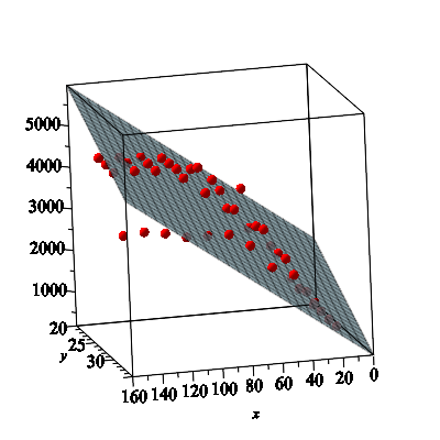
The length of a species of fish is to be represented as a function of the age and water temperature as shown in the table on the next page.⁴⁷ The fish are kept in tanks at 25, 27, 29 and 31 degrees Celsius. After birth, a test specimen is chosen at random every 14 days and its length measured. The data include:

$I,$ the index;
$x,$ the age of the fish in days;
$y,$ the water temperature in degrees Celsius;
$z,$ the length of the fish.

Since there are three variables in the data, we cannot perform a simple linear regression. Instead, we seek a model of the form

f (x, y) = a x + b y + c

to fit the data, where $f (x, y)$ approximates the length. That is, we seek the best fit plane to the data. This is an example of what is called multiple linear regression. A scatterplot of the data, along with the best fit plane, is also shown.

🔗

(a)

As we did when we fit polynomials to data, we start by considering what would happen if all of our data points satisfied our model function. In this case our data points have the form $(x_{1}, y_{1}, z_{1}),$ $(x_{2}, y_{2}, z_{2}),$ $\dots,$ $(x_{m}, y_{m}, z_{m}) .$ Explain what system of linear equations would result if the data points actually satisfy our model function $f (x, y) = a x + b y + c .$ (You don't need to write 44 different equations, just explain the general form of the system.)

🔗

(b)

Write the system from (a) in the form $M a = z,$ and specifically identify the matrix $M$ and the vectors $a$ and $z .$

🔗

(c)

The same derivation as with the polynomial regression models shows that the vector $a^{*}$ that minimizes $| | z - M a | |$ is found by

a^{*} = {(M^{T} M)}^{- 1} M^{T} z,

Use this to find the least squares fit of the form $f (x, y) = a x + b y + c$ to the data.

🔗

(d)

Provide a numeric measure of how well this model function fits the data. Explain.

Index	Age	Temp ( $^{\circ}$ C)	Length
1	14	25	620
2	28	25	1315
3	41	25	2120
4	55	25	2600
5	69	25	3110
6	83	25	3535
7	97	25	3935
8	111	25	4465
9	125	25	4530
10	139	25	4570
11	153	25	4600
12	14	27	625
13	28	27	1215
14	41	27	2110
15	55	27	2805
16	69	27	3255
17	83	27	4015
18	97	27	4315
19	111	27	4495
20	125	27	4535
21	139	27	4600
22	153	27	4600
23	14	29	590
24	28	29	1305
25	41	29	2140
26	55	29	2890
27	69	29	3920
28	83	29	3920
29	97	29	4515
30	111	29	4520
31	125	29	4525
32	139	29	4565
33	153	29	4566
34	14	31	590
35	28	31	1205
36	41	31	1915
37	55	31	2140
38	69	31	2710
39	83	31	3020
40	97	31	3030
41	111	31	3040
42	125	31	3180
43	139	31	3257
44	153	31	3214

🔗

Project Activity 26.6.

Population growth is typically not well modeled by polynomial functions. Populations tend to grow at rates proportional to the population, which implies exponential growth. For example, Table 26.16 shows the approximate population of the United States in years between 1920 and 2000, with the population measured in millions.

Table 26.16. U.S. population

Year	1920	1930	1940	1950	1960	1970	1980	1990	2000
Population	106	123	142	161	189	213	237	259	291

If we assume the population grows exponentially, we would want to find the best fit function $f$ of the form $f (t) = a e^{k t},$ where $a$ and $k$ are constants. However, an exponential function is not linear. So to apply the methods we have developed, we could instead apply the natural logarithm to both sides of $y = a e^{k t}$ to obtain the equation $\ln (y) = \ln (a) + k t .$ We can then find the best fit line to the data in the form $(t, \ln (y))$ to determine the values of $\ln (a)$ and $k .$ Use this approach to find the best fit exponential function in the least squares sense to the U.S. population data. Then look up the U.S. population in 2010 (include your source) and compare to the estimate given by your model function. If your prediction is not very close, give some plausible explanations for the difference.

🔗

Project Activity 26.7.

Carl Friedrich Gauss is often credited with inventing the method of least squares. He used the method to find a best-fit ellipse which allowed him to correctly predict the orbit of the asteroid Ceres as it passed behind the sun in 1801. (Adrien-Marie Legendre appears to be the first to publish the method, though.) Here we examine the problem of fitting an ellipse to data.

An ellipse is a quadratic equation that can be written in the form

\begin{matrix} (26.10) & x^{2} + B y^{2} + C x y + D x + E y + F = 0 \end{matrix}

for constants $B,$ $C,$ $D,$ $E,$ and $F,$ with $B > 0 .$ We will find the best-fit ellipse in the least squares sense through the points

(0, 2), (2, 1), (1, - 1), (- 1, - 2), (- 3, 1), and (- 1, - 1) .

A picture of the best fit ellipse is shown in Figure 26.17.

🔗

(a)

Find the system of linear equations that would result if the ellipse (26.10) were to exactly pass through the given points.

🔗

(b)

Write the linear system from part (a) in the form $A x = b,$ where the vector $x$ contains the unknowns in the system. Clearly identify $A,$ $x,$ and $b .$

🔗

(c)

Find the least squares ellipse to this set of points. Make sure your method is clear. (Note that we are really fitting a surface of the form $f (x, y) = x^{2} + B y^{2} + C x y + D x + E y + F$ to a set of data points in the $x y$ -plane. So the error is the sum of the vertical distances from the points in the $x y$ -plane to the surface.)

cdc.gov/growthcharts/html_charts/lenageinf.htm

macrotrends.net/countries/USA/united-states/life-expectancy

Data from Mathematical Algorithms for Linear Regression, Helmut Spaeth, Academic Press, 1991, page 305, ISBN 0-12-656460-4.