Using the Singular Value Decomposition

Section 30 Using the Singular Value Decomposition

Focus Questions

By the end of this section, you should be able to give precise and thorough answers to the questions listed below. You may want to keep these questions in mind to focus your thoughts as you complete the section.

What is the condition number of a matrix and what does it tell us about the matrix?
What is the pseudoinverse of a matrix?
Why are pseudoinverses useful?
How does the pseudoinverse of a matrix allow us to find least squares solutions to linear systems?

🔗

Subsection Application: Global Positioning System

🔗

You are probably familiar with the Global Positioning System (GPS). The system allows anyone with the appropriate software to accurately determine their location at any time. The applications are almost endless, including getting real-time driving directions while in your car, guiding missiles, and providing distances on golf courses.

🔗

The GPS is a worldwide radio-navigation system owned by the US government and operated by the US Air Force. GPS is one of four global navigation satellite systems. At least twenty four GPS satellites orbit the Earth at an altitude of approximately 11,000 nautical miles. The satellites are placed so that at any time at least four of them can be accessed by a GPS receiver. Each satellite carries an atomic clock to relay a time stamp along with its position in space. There are five ground stations to coordinate and ensure that the system is working properly.

🔗

The system works by triangulation, but there is also error involved in the measurements that go into determining position. Later in this section we will see how the method of least squares can be used to determine the receiver's position.

🔗

Subsection Introduction

🔗

A singular value decomposition has many applications, and in this section we discuss how a singular value decomposition can be used in image compression, to determine how sensitive a matrix can be to rounding errors in the process of row reduction, and to solve least squares problems.

🔗

Subsection Image Compression

🔗

The digital age has brought many new opportunities for the collection, analysis, and dissemination of information. Along with these opportunities come new difficulties as well. All of this digital information must be stored in some way and be retrievable in an efficient manner. A singular value decomposition of digitally stored information can be used to compress the information or clean up corrupted information. In this section we will see how a singular value decomposition can be used in image compression. While a singular value decomposition is normally used with very large matrices, we will restrict ourselves to small examples so that we can more clearly see how a singular value decomposition is applied.

🔗

Preview Activity 30.1.

Let $A = \frac{1}{4} [\begin{array}{ccrr} 67 & 29 & - 31 & - 73 \\ 29 & 67 & - 73 & - 31 \\ 31 & 73 & - 67 & - 29 \\ 73 & 31 & - 29 & - 67 \end{array}] .$ A singular value decomposition for $A$ is $U Σ V^{T},$ where

\begin{aligned} U & = [u_{1} u_{2} u_{3} u_{4}] = \frac{1}{2} [\begin{array}{crrr} 1 & - 1 & 1 & - 1 \\ 1 & 1 & 1 & 1 \\ 1 & 1 & - 1 & - 1 \\ 1 & - 1 & - 1 & 1 \end{array}], \\ Σ & = [\begin{array}{cccc} 50 & 0 & 0 & 0 \\ 0 & 20 & 0 & 0 \\ 0 & 0 & 2 & 0 \\ 0 & 0 & 0 & 1 \end{array}], \\ V & = [v_{1} v_{2} v_{3} v_{4}] = \frac{1}{2} [\begin{array}{rrrr} 1 & 1 & - 1 & 1 \\ 1 & - 1 & - 1 & - 1 \\ - 1 & 1 & - 1 & - 1 \\ - 1 & - 1 & - 1 & 1 \end{array}] . \end{aligned}

🔗

(a)

Write the summands in the corresponding outer product decomposition of $A .$

🔗

(b)

The outer product decomposition of $A$ writes $A$ as a sum of rank 1 matrices (the summands $σ_{i} u_{i} v_{i}^{T}) .$ Each summand contains some information about the matrix $A .$ Since $σ_{1}$ is the largest of the singular values, it is reasonable to expect that the summand $A_{1} = σ_{1} u_{1} v_{1}^{T}$ contains the most information about $A$ among all of the summands. To get a measure of how much information $A_{1}$ contains of $A,$ we can think of $A$ as simply a long vector in $R^{m n}$ where we have folded the data into a rectangular array (we will see later why taking the norm as the norm of the vector in $R^{n m}$ makes sense, but for now, just use this definition). If we are interested in determining the error in approximating an image by a compressed image, it makes sense to use the standard norm in $R^{m n}$ to determine length and distance, which is really just the Frobenius norm that comes from the Frobenius inner product defined by

\begin{matrix} (30.1) & ⟨ U, V ⟩ = \sum u_{i j} v_{i j}, \end{matrix}

where $U = [u_{i j}]$ and $V = [v_{i j}]$ are $m \times n$ matrices. (That (30.1) defines an inner product on the set of all $n \times n$ matrices is left to discuss in a later section.) So in this section all the norms for matrices will refer to the Frobenius norm. Rather than computing the distance between $A_{1}$ and $A$ to measure the error, we are more interested in the relative error

\frac{| | A - A_{1} | |}{| | A | |} .

🔗

(i)

Calculate the relative error in approximating $A$ by $A_{1} .$ What does this tell us about how much information $A_{1}$ contains about $A ?$

🔗

(ii)

Let $A_{2} = \sum_{k = 1}^{2} σ_{k} u_{k} v_{k}^{T} .$ Calculate the relative error in approximating $A$ by $A_{2} .$ What does this tell us about how much information $A_{2}$ contains about $A ?$

🔗

(iii)

Let $A_{3} = \sum_{k = 1}^{3} σ_{k} u_{k} v_{k}^{T} .$ Calculate the relative error in approximating $A$ by $A_{3} .$ What does this tell us about how much information $A_{3}$ contains about $A ?$

🔗

(iv)

Let $A_{4} = \sum_{k = 1}^{4} σ_{k} u_{k} v_{k}^{T} .$ Calculate the relative error in approximating $A$ by $A_{4} .$ What does this tell us about how much information $A_{4}$ contains about $A ?$ Why?

🔗

The first step in compressing an image is to digitize the image. There are many ways to do this and we will consider one of the simplest ways and only work with gray-scale images, with the scale from 0 (black) to 255 (white). A digital image can be created by taking a small grid of squares (called pixels) and coloring each pixel with some shade of gray. The resolution of this grid is a measure of how many pixels are used per square inch. As an example, consider the 16 by 16 pixel picture of a flower shown in Figure 30.1.

🔗

To store this image pixel by pixel would require

16 \times 16 = 256

units of storage space (1 for each pixel). If we let

M

be the matrix whose

i, j

th entry is the scale of the

i, j

th pixel, then

M

is the matrix

[\begin{array}{cccccccccccccccc} 240 & 240 & 240 & 240 & 130 & 130 & 240 & 130 & 130 & 240 & 240 & 240 & 240 & 240 & 240 & 240 \\ 240 & 240 & 240 & 130 & 175 & 175 & 130 & 175 & 175 & 130 & 240 & 240 & 240 & 240 & 240 & 240 \\ 240 & 240 & 130 & 130 & 175 & 175 & 130 & 175 & 175 & 130 & 130 & 240 & 240 & 240 & 240 & 240 \\ 240 & 130 & 175 & 175 & 130 & 175 & 175 & 175 & 130 & 175 & 175 & 130 & 240 & 240 & 240 & 240 \\ 240 & 240 & 130 & 175 & 175 & 130 & 175 & 130 & 175 & 175 & 130 & 240 & 240 & 240 & 240 & 240 \\ 255 & 240 & 240 & 130 & 130 & 175 & 175 & 175 & 130 & 130 & 240 & 240 & 225 & 240 & 240 & 240 \\ 240 & 240 & 130 & 175 & 175 & 130 & 130 & 130 & 175 & 175 & 130 & 240 & 225 & 255 & 240 & 240 \\ 240 & 240 & 130 & 175 & 130 & 240 & 130 & 240 & 130 & 175 & 130 & 240 & 255 & 255 & 255 & 240 \\ 240 & 240 & 240 & 130 & 240 & 240 & 75 & 240 & 240 & 130 & 240 & 255 & 255 & 255 & 255 & 255 \\ 240 & 240 & 240 & 240 & 240 & 240 & 75 & 240 & 240 & 240 & 240 & 240 & 240 & 240 & 240 & 240 \\ 240 & 240 & 240 & 75 & 75 & 240 & 75 & 240 & 75 & 75 & 240 & 240 & 240 & 240 & 240 & 240 \\ 50 & 240 & 240 & 240 & 75 & 240 & 75 & 240 & 75 & 240 & 240 & 240 & 240 & 50 & 240 & 240 \\ 240 & 75 & 240 & 240 & 240 & 75 & 75 & 75 & 240 & 240 & 50 & 240 & 50 & 240 & 240 & 50 \\ 240 & 240 & 75 & 240 & 240 & 240 & 75 & 240 & 240 & 50 & 240 & 50 & 240 & 240 & 50 & 240 \\ 75 & 75 & 75 & 75 & 75 & 75 & 75 & 75 & 75 & 75 & 75 & 75 & 75 & 75 & 75 & 75 \\ 75 & 75 & 75 & 75 & 75 & 75 & 75 & 75 & 75 & 75 & 75 & 75 & 75 & 75 & 75 & 75 \end{array}] .

🔗

Recall that if

U Σ V^{T}

is a singular value decomposition for

M,

then we can also write

M

in the form

M = σ_{1} u_{1} v_{1}^{T} + σ_{2} u_{2} v_{2}^{T} + σ_{3} u_{3} v_{3}^{T} + \dots + σ_{16} u_{16} v_{16}^{T} .

🔗

given in (29.2). For this

M,

the singular values are approximately

\begin{matrix} (30.2) & [\begin{matrix} 3006.770088367795 \\ 439.13109000200205 \\ 382.1756550649652 \\ 312.1181752764884 \\ 254.45105800344953 \\ 203.36470770057494 \\ 152.8696215072527 \\ 101.29084240890717 \\ 63.80803769229468 \\ 39.6189181773536 \\ 17.091891798245463 \\ 12.304589419140656 \\ 4.729898943556077 \\ 2.828719409809012 \\ 6.94442317024232 \times 10^{- 15} \\ 2.19689952047833 \times 10^{- 15} \end{matrix}] . \end{matrix}

🔗

Notice that some of these singular values are very small compared to others. As in Preview Activity 30.1, the terms with the largest singular values contain most of the information about the matrix. Thus, we shouldn't lose much information if we eliminate the small singular values. In this particular example, the last 4 singular values are significantly smaller than the rest. If we let

M_{12} = σ_{1} u_{1} v_{1}^{T} + σ_{2} u_{2} v_{2}^{T} + σ_{3} u_{3} v_{3}^{T} + \dots + σ_{12} u_{12} v_{12}^{T},

🔗

then we should expect the image determined by

M_{12}

to be close to the image made by

M .

The two images are presented side by side in Figure 30.2.

🔗
Figure 30.2. A 16 by 16 pixel image and a compressed image using a singular value decomposition.

🔗

This small example illustrates the general idea. Suppose we had a satellite image that was

1000 \times 1000

pixels and we let

M

represent this image. If we have a singular value decomposition of this image

M,

say

M = σ_{1} u_{1} v_{1}^{T} + σ_{2} u_{2} v_{2}^{T} + σ_{3} u_{3} v_{3}^{T} + \dots + σ_{r} u_{r} v_{r}^{T},

🔗

if the rank of

M

is large, it is likely that many of the singular values will be very small. If we only keep

s

of the singular values, we can approximate

M

M_{s} = σ_{1} u_{1} v_{1}^{T} + σ_{2} u_{2} v_{2}^{T} + σ_{3} u_{3} v_{3}^{T} + \dots + σ_{s} u_{s} v_{s}^{T}

🔗

and store the image with only the vectors

σ_{1} u_{1},

σ_{2} u_{2},

\dots,

σ_{s} u_{s},

v_{1},

v_{1},

\dots,

v_{s} .

For example, if we only need 10 of the singular values of a satellite image (

s = 10

), then we can store the satellite image with only 20 vectors in

R^{1000}

or with

20 \times 1000 = 20, 000

numbers instead of

1000 \times 1000 = 1, 000, 000

numbers.

🔗

A similar process can be used to denoise data.⁵²

🔗

Subsection Calculating the Error in Approximating an Image

🔗

In the context where a matrix represents an image, the operator aspect of the matrix is irrelevant — we are only interested in the matrix as a holder of information. In this situation, we think of an

m \times n

matrix as simply a long vector in

R^{m n}

where we have folded the data into a rectangular array. If we are interested in determining the error in approximating an image by a compressed image, it makes sense to use the standard norm in

R^{m n}

to determine length and distance. This leads to what is called the Frobenius norm of a matrix. The Frobenius norm

| | M | |_{F}

of an

m \times n

matrix

M = [m_{i j}]

| | M | |_{F} = \sqrt{\sum m_{i j}^{2}} .

🔗

There is a natural corresponding inner product on the set of

m \times n

matrices (called the Frobenius product) defined by

⟨ A, B ⟩ = \sum a_{i j} b_{i j},

🔗

where

A = [a_{i j}]

and

B = [b_{i j}]

are

m \times n

matrices. Note that

| | A | |_{F} = \sqrt{⟨ A, A ⟩} .

🔗

If an

m \times n

matrix

M

of rank

r

has a singular value decomposition

M = U Σ V^{T},

we have seen that we can write

M

as an outer product

\begin{matrix} (30.3) & M = σ_{1} u_{1} v_{1}^{T} + σ_{2} u_{2} v_{2}^{T} + σ_{3} u_{3} v_{3}^{T} + \dots + σ_{r} u_{r} v_{r}^{T}, \end{matrix}

🔗

where the

u_{i}

are the columns of

U

and the

v_{j}

the columns of

V .

Each of the products

u_{i} v_{i}^{T}

is an

m \times n

matrix. Since the columns of

u_{i} v_{i}^{T}

are all scalar multiples of

u_{i},

the matrix

u_{i} v_{i}^{T}

is a rank 1 matrix. So (30.3) expresses

M

as a sum of rank 1 matrices. Moreover, if we let

x

and

w

m \times 1

vectors and let

y

and

z

n \times 1

vectors with

y = [y_{1} y_{2} \dots y_{n}]^{T}

and

z = [z_{1} z_{2} \dots z_{n}]^{T},

then

\begin{aligned} ⟨ x y^{T}, w z^{T} ⟩ & = ⟨ [y_{1} x y_{2} x \dots y_{n} x], [z_{1} w z_{2} w \dots z_{n} w] ⟩ \\ = \sum (y_{i} x) \cdot (z_{i} w) \\ = \sum (y_{i} z_{i}) (x \cdot w) \\ = (x \cdot w) \sum (y_{i} z_{i}) \\ = (x \cdot w) (y \cdot z) . \end{aligned}

🔗

Using the vectors from the singular value decomposition of

M

as in (30.3) we see that

⟨ u_{i} v_{i}^{T}, u_{j} v_{j}^{T} ⟩ = (u_{i} \cdot u_{j}) (v_{i} \cdot v_{j}) = {\begin{cases} 0, & if i \neq j, \\ 1, & if i = j . \end{cases}

🔗

It follows that

\begin{matrix} (30.4) & | | M | |_{F}^{2} = \sum σ_{i}^{2} (u_{i} \cdot u_{i}) (v_{i} \cdot v_{i}) = \sum σ_{i}^{2} . \end{matrix}

🔗

Activity 30.2.

Verify (30.4) that $| | M | |_{F}^{2} = \sum σ_{i}^{2} .$

🔗

When we used the singular value decomposition to approximate the image defined by

M,

we replaced

M

with a matrix of the form

\begin{matrix} (30.5) & M_{k} = σ_{1} u_{1} v_{1}^{T} + σ_{2} u_{2} v_{2}^{T} + σ_{3} u_{3} v_{3}^{T} + \dots + σ_{k} u_{k} v_{k}^{T} . \end{matrix}

🔗

We call

M_{k}

the rank

k

approximation to

M .

Notice that the outer product expansion in (30.5) is in fact a singular value decomposition for

M_{k} .

The error

E_{k}

in approximating

M

with

M_{k}

\begin{matrix} (30.6) & E_{k} = M - M_{k} = σ_{k + 1} u_{k + 1} v_{k + 1}^{T} + σ_{k + 2} u_{k + 2} v_{k + 2}^{T} + \dots + σ_{r} u_{r} v_{r}^{T} . \end{matrix}

🔗

Once again, notice that (30.6) is a singular value decomposition for

E_{k} .

We define the relative error in approximating

M

with

M_{k}

\frac{| | E_{k} | |}{| | M | |} .

🔗

Now (30.4) shows that

\frac{| | E_{k} | |}{| | M | |} = \sqrt{\frac{\sum_{i = k + 1}^{r} σ_{i}^{2}}{\sum_{i = 1}^{r} σ_{i}^{2}}} .

🔗

In applications, we often want to retain a certain degree of accuracy in our approximations and this error term can help us accomplish that.

🔗

In our flower example, the singular values of

M

are given in (30.2). The relative error in approximating

M

with

M_{12}

\sqrt{\frac{\sum_{i = 13}^{16} σ_{i}^{2}}{\sum_{i = 1}^{16} σ_{i}^{2}}} \approx 0.0018 .

🔗

Errors (rounded to 4 decimal places) for approximating

M

with some of the

M_{k}

are shown in Table 30.3

🔗

Table 30.3. Errors in approximating

M

M_{k}

$k$	10	9	8	7	6
$\frac{\| \| E_{k} \| \|}{\| \| M \| \|}$	0.0070	0.0146	0.0252	0.0413	0.06426
$k$	5	4	3	2	1
$\frac{\| \| E_{k} \| \|}{\| \| M \| \|}$	0.0918	0.1231	0.1590	0.201	0.2460

🔗

Activity 30.3.

Let $M$ represent the flower image.

🔗

(a)

Find the relative errors in approximating $M$ by $M_{13}$ and $M_{14} .$ You may use the fact that $\sqrt{\sum_{i = 1}^{16} σ_{i}^{2}} \approx 3102.0679 .$

🔗

(b)

About how much of the information in the image is contained in the rank 1 approximation? Explain.

🔗

Subsection The Condition Number of a Matrix

🔗

A singular value decomposition for a matrix

A

can tell us a lot about how difficult it is to accurately solve a system

A x = b .

Solutions to systems of linear equations can be very sensitive to rounding as the next exercise demonstrates.

🔗

Activity 30.4.

Find the solution to each of the systems.

🔗

(a)

$[\begin{array}{cc} 1.0000 & 1.0000 \\ 1.0000 & 1.0005 \end{array}] [\begin{matrix} x \\ y \end{matrix}] = [\begin{matrix} 2.0000 \\ 2.0050 \end{matrix}]$

🔗

(b)

$[\begin{array}{cc} 1.000 & 1.000 \\ 1.000 & 1.001 \end{array}] [\begin{matrix} x \\ y \end{matrix}] = [\begin{matrix} 2.000 \\ 2.005 \end{matrix}]$

🔗

Notice that a simple rounding in the

(2, 2)

entry of the coefficient matrix led to a significantly different solution. If there are rounding errors at any stage of the Gaussian elimination process, they can be compounded by further row operations. This is an important problem since computers can only approximate irrational numbers with rational numbers and so rounding can be critical. Finding ways of dealing with these kinds of errors is an area of on-going research in numerical linear algebra. This problem is given a name.

🔗

Definition 30.4.

A matrix $A$ is ill-conditioned if relatively small changes in any entries of $A$ can produce significant changes in solutions to the system $A x = b .$

🔗

A matrix that is not ill-conditioned is said to be well-conditioned. Since small changes in entries of ill-conditioned matrices can lead to large errors in computations, it is an important problem in linear algebra to have a way to measure how ill-conditioned a matrix is. This idea will ultimately lead us to the condition number of a matrix.

🔗

Suppose we want to solve the system

A x = b,

where

A

is an invertible matrix. Activity 30.4 illustrates that if

A

is really close to being singular, then small changes in the entries of

A

can have significant effects on the solution to the system. So the system can be very hard to solve accurately if

A

is close to singular. It is important to have a sense of how “good” we can expect any calculated solution to be. Suppose we think we solve the system

A x = b

but, through rounding error in our calculation of

A,

get a solution

x^{'}

so that

A x^{'} = b^{'},

where

b^{'}

is not exactly

b .

Let

Δ x

be the error in our calculated solution and

Δ b

the difference between

b^{'}

and

b .

We would like to know how large the error

| | Δ x | |

can be. But this isn't exactly the right question. We could scale everything to make

| | Δ x | |

as large as we want. What we really need is a measure of the relative error

\frac{| | Δ x | |}{| | x | |},

or how big the error is compared to

| | x | |

itself. More specifically, we want to know how large the relative error in

Δ x

is compared to the relative error in

Δ b .

In other words, we want to know how good the relative error in

Δ b

is as a predictor of the relative error in

Δ x

(we may have some control over the relative error in

Δ b,

perhaps by keeping more significant digits). So we want know if there is a best constant

C

such that

\frac{| | Δ x | |}{| | x | |} \leq C \frac{| | Δ b | |}{| | b | |} .

🔗

This best constant

C

is the condition number — a measure of how well the relative error in

Δ b

predicts the relative error in

Δ x .

How can we find

C ?

🔗

Since

A x^{'} = b^{'}

we have

A (x + Δ x) = b + Δ b .

🔗

Distributing on the left and using the fact that

A x = b

gives us

\begin{matrix} (30.7) & A Δ x = Δ b . \end{matrix}

🔗

We return for a moment to the operator norm of a matrix. This is an appropriate norm to use here since we are considering

A

to be a transformation. Recall that if

A

is an

m \times n

matrix, we defined the operator norm of

A

to be

| | A | | = max_{| | x | | \neq 0} {\frac{| | A x | |}{| | x | |}} = max_{| | x | | = 1} {| | A x | |} .

🔗

One important property that the norm has is that if the product

A B

is defined, then

| | A B | | \leq | | A | | | | B | | .

🔗

To see why, notice that

\frac{| | A B x | |}{| | x | |} = \frac{| | A (B x) | |}{| | B x | |} \frac{| | B x | |}{| | x | |} .

🔗

Now

\frac{| | A (B x) | |}{| | B x | |} \leq | | A | |

and

\frac{| | B x | |}{| | x | |} \leq | | B | |

by the definition of the norm, so we conclude that

\frac{| | A B x | |}{| | x | |} \leq | | A | | | | B | |

🔗

for every

x .

Thus,

| | A B | | \leq | | A | | | | B | | .

🔗

Now we can find the condition number. From

A Δ x = Δ b

we have

Δ x = A^{- 1} Δ b,

🔗

\begin{matrix} (30.8) & | | Δ x | | \leq | | A^{- 1} | | | | Δ b | | . \end{matrix}

🔗

Similarly,

b = A x

implies that

| | b | | \leq | | A | | | | x | |

\begin{matrix} (30.9) & \frac{1}{| | x | |} \leq \frac{| | A | |}{| | b | |} . \end{matrix}

🔗

Combining (30.8) and (30.9) gives

\begin{aligned} \frac{| | Δ x | |}{| | x | |} & \leq \frac{| | A^{- 1} | | | | Δ b | |}{| | x | |} \\ = | | A^{- 1} | | | | Δ b | | (\frac{1}{| | x | |}) \\ \leq | | A^{- 1} | | | | Δ b | | \frac{| | A | |}{| | b | |} \\ = | | A^{- 1} | | | | A | | \frac{| | Δ b | |}{| | b | |} . \end{aligned}

🔗

This constant

| | A^{- 1} | | | | A | |

is the best bound and so is called the condition number of

A .

🔗

Definition 30.5.

The condition number of an invertible matrix $A$ is the number $| | A^{- 1} | | | | A | | .$

🔗

How does a singular value decomposition tell us about the condition number of a matrix? Recall that the maximum value of

| | A x | |

for

x

on the unit

n

-sphere is

σ_{1} .

| | A | | = σ_{1} .

A

is an invertible matrix and

A = U Σ V^{T}

is a singular value decomposition for

A,

then

A^{- 1} = (U Σ V^{T})^{- 1} = (V^{T})^{- 1} Σ^{- 1} U^{- 1} = V Σ^{- 1} U^{T},

🔗

where

Σ^{- 1} = [\begin{array}{ccccc} \frac{1}{σ_{1}} & 0 \\ \frac{1}{σ_{2}} \\ \frac{1}{σ_{3}} \\ ⋱ \\ 0 & \frac{1}{σ_{n}} \end{array}] .

🔗

Now

V Σ^{- 1} U^{T}

is a singular value decomposition for

A^{- 1}

with the diagonal entries in reverse order, so

| | A^{- 1} | | = \frac{1}{σ_{n}} .

🔗

Therefore, the condition number of

A

| | A^{- 1} | | | | A | | = \frac{σ_{1}}{σ_{n}} .

🔗

Activity 30.5.

Let $A = [\begin{array}{cc} 1.0000 & 1.0000 \\ 1.0000 & 1.0005 \end{array}] .$ A computer algebra system gives the singular values of $A$ as 2.00025003124999934 and 0.000249968750000509660. What is the condition number of $A .$ What does that tell us about $A ?$ Does this seem reasonable given the result of Activity 30.4?

🔗

Activity 30.6.

🔗

(a)

What is the smallest the condition number of a matrix can be? Find an entire class of matrices with this smallest condition number.

🔗

(b)

What is the condition number of an orthogonal matrix? Why does this make sense?

Hint.

If $P$ is an orthogonal matrix, what is $| | P x | |$ for any vector $x ?$ What does this make $| | P | | ?$

🔗

(c)

What is the condition number of an invertible symmetric matrix in terms of its eigenvalues?

🔗

(d)

Why do we not define the condition number of a non-invertible matrix? If we did, what would the condition number have to be? Why?

🔗

Subsection Pseudoinverses

🔗

Not every matrix is invertible, so we cannot always solve a matrix equation

A x = b .

However, every matrix has a pseudoinverse

A^{+}

that acts something like an inverse. Even when we can't solve a matrix equation

A x = b

because

b

isn't in

Col A,

we can use the pseudoinverse of

A

to “solve” the equation

A x = b

with the “solution”

A^{+} b .

While not an exact solution,

A^{+} b

turns out to be the best approximation to a solution in the least squares sense. We will use the singular value decomposition to find the pseudoinverse of a matrix.

🔗

Preview Activity 30.7.

Let $A = [\begin{array}{ccc} 1 & 1 & 0 \\ 0 & 1 & 1 \end{array}] .$ The singular value decomposition of $A$ is $U Σ V^{T}$ where

\begin{aligned} U & = \frac{\sqrt{2}}{2} [\begin{array}{cr} 1 & - 1 \\ 1 & 1 \end{array}], \\ Σ & = [\begin{array}{ccc} \sqrt{3} & 0 & 0 \\ 0 & 1 & 0 \end{array}], \\ V & = \frac{1}{6} [\begin{array}{rrr} \sqrt{6} & - 3 \sqrt{2} & 2 \sqrt{3} \\ 2 \sqrt{6} & 0 & - 2 \sqrt{3} \\ \sqrt{6} & 3 \sqrt{2} & 2 \sqrt{3} \end{array}] . \end{aligned}

🔗

(a)

Explain why $A$ is not an invertible matrix.

🔗

(b)

Explain why the matrices $U$ and $V$ are invertible. How are $U^{- 1}$ and $V^{- 1}$ related to $U^{T}$ and $V^{T} ?$

🔗

(c)

Recall that one property of invertible matrices is that the inverse of a product of invertible matrices is the product of the inverses in the reverse order. If $A$ were invertible, then $A^{- 1}$ would be ${(U Σ V^{T})}^{- 1} = V Σ^{- 1} U^{T} .$ Even though $U$ and $V$ are invertible, the matrix $Σ$ is not. But $Σ$ does contain non-zero eigenvalues that have reciprocals, so consider the matrix $Σ^{+} = [\begin{array}{cc} \frac{1}{\sqrt{3}} & 0 \\ 0 & 1 \\ 0 & 0 \end{array}] .$ Calculate the products $Σ Σ^{+}$ and $Σ^{+} Σ .$ How are the results similar to that obtained with a matrix inverse?

🔗

(d)

The only matrix in the singular value decomposition of $A$ that is not invertible is $Σ .$ But the matrix $Σ^{+}$ acts somewhat like an inverse of $Σ,$ so let us define $A^{+}$ as $V Σ^{+} U^{T} .$ Now we explore a few properties of the matrix $A^{+} .$

🔗

(i)

Calculate $A A^{+}$ and $A^{+} A$ for $A = [\begin{array}{ccc} 1 & 1 & 0 \\ 0 & 1 & 1 \end{array}] .$ What do you notice?

🔗

(ii)

Calculate $A^{+} A A^{+}$ and $A A^{+} A$ for $A = [\begin{array}{ccc} 1 & 1 & 0 \\ 0 & 1 & 1 \end{array}] .$ What do you notice?

🔗

Only some square matrices have inverses. However, every matrix has a pseudoinverse. A pseudoinverse

A^{+}

of a matrix

A

provides something like an inverse when a matrix doesn't have an inverse. Pseudoinverses are useful to approximate solutions to linear systems. If

A

is invertible, then the equation

A x = b

has the solution

x = A^{- 1} b,

but when

A

is not invertible and

b

is not in

Col A,

then the equation

A x = b

has no solution. In the invertible case of an

n \times n

matrix

A,

there is a matrix

B

so that

A B = B A = I_{n} .

This also implies that

B A B = B

and

A B A = A .

To mimic this situation when

A

is not invertible, we search for a matrix

A^{+}

(a pseudoinverse of

A

) so that

A A^{+} A = A

and

A^{+} A A^{+} = A^{+},

as we saw in Preview Activity 30.7. Then it turns out that

A^{+}

acts something like an inverse for

A .

In this case, we approximate the solution to

A x = b

x^{*} = A^{+} b,

and we will see that the vector

A x^{*} = A A^{+} b

turns out to be the vector in

Col A

that is closest to

b

in the least squares sense.

🔗

A reasonable question to ask is how we can find a pseudoinverse of a matrix

A .

A singular value decomposition provides an answer to this question. If

A

is an invertible

n \times n

matrix, then 0 is not an eigenvalue of

A .

As a result, in the singular value decomposition

U Σ V^{T}

A,

the matrix

Σ

is an invertible matrix (note that

U,

Σ,

and

V

are all

n \times n

matrices in this case). So

A^{- 1} = {(U Σ V^{T})}^{- 1} = V Σ^{- 1} U^{T},

🔗

where

Σ^{- 1} = [\begin{array}{ccccc} \frac{1}{σ_{1}} \\ \frac{1}{σ_{2}} & 0 \\ \frac{1}{σ_{3}} \\ 0 & ⋱ \\ \frac{1}{σ_{n}} \end{array}] .

🔗

In this case,

V Σ^{- 1} U^{T}

is a singular value decomposition for

A^{- 1} .

🔗

To understand in general how a pseudoinverse is found, let

A

be an

m \times n

matrix with

m \neq n,

or an

n \times n

with rank less than

n .

In these cases

A

does not have an inverse. But as in Preview Activity 30.7, a singular value decomposition provides a pseudoinverse

A^{+}

for

A .

Let

U Σ V^{T}

be a singular value decomposition of an

m \times n

matrix

A

of rank

r,

with

Σ = [\begin{array}{cccccc} σ_{1} \\ σ_{2} & 0 & 0 \\ σ_{3} \\ 0 & ⋱ \\ σ_{r} \\ 0 & 0 \end{array}]

🔗

The matrices

U

and

V

are invertible, but the matrix

Σ

is not if

A

is not invertible. If we let

Σ^{+}

be the

n \times m

matrix defined by

Σ^{+} = [\begin{array}{cccccc} \frac{1}{σ_{1}} \\ \frac{1}{σ_{2}} & 0 & 0 \\ \frac{1}{σ_{3}} \\ 0 & ⋱ \\ \frac{1}{σ_{r}} \\ 0 & 0 \end{array}],

🔗

then

Σ^{+}

will act much like an inverse of

Σ

might. In fact, it is not difficult to see that

Σ Σ^{+} = [\begin{array}{cc} I_{r} & 0 \\ 0 & 0 \end{array}] and Σ^{+} Σ = [\begin{array}{cc} I_{r} & 0 \\ 0 & 0 \end{array}],

🔗

where

Σ Σ^{+}

is an

m \times m

matrix and

Σ^{+} Σ

is an

n \times n

matrix.

🔗

The matrix

\begin{matrix} (30.10) & A^{+} = V Σ^{+} U^{T} \end{matrix}

🔗

is a pseudoinverse of

A .

🔗

Activity 30.8.

🔗

(a)

Find the pseudoinverse $A^{+}$ of $A = [\begin{array}{rc} 0 & 5 \\ 4 & 3 \\ - 2 & 1 \end{array}] .$ Use the singular value decomposition $U Σ V^{T}$ of $A,$ where

U = [\begin{array}{crc} \frac{\sqrt{2}}{2} & \frac{\sqrt{3}}{3} & 1 \\ \frac{\sqrt{2}}{2} & - \frac{\sqrt{3}}{3} & 0 \\ 0 & \frac{\sqrt{3}}{3} & 0 \end{array}], Σ = [\begin{array}{cc} \sqrt{40} & 0 \\ 0 & \sqrt{15} \\ 0 & 0 \end{array}], V = \frac{1}{\sqrt{5}} [\begin{array}{cr} 1 & - 2 \\ 2 & 1 \end{array}] .

🔗

(b)

The vector $b = [\begin{matrix} 0 \\ 0 \\ 1 \end{matrix}]$ is not in $Col A .$ The vector $x^{*} = A^{+} b$ is an approximation to a solution of $A x = b,$ and $A A^{+} b$ is in $Col A .$ Find $A x^{*}$ and determine how far $A x^{*}$ is from $b .$

🔗

Pseudoinverses satisfy several properties that are similar to those of inverses. For example, we had an example in Preview Activity 30.7 where

A A^{+} A = A

and

A^{+} A A^{+} = A^{+} .

That

A^{+}

always satisfies these properties is the subject of the next activity.

🔗

Activity 30.9.

Let $A$ be an $m \times n$ matrix with singular value decomposition $U Σ V^{T} .$ Let $A^{+}$ be defined as in (30.10).

🔗

(a)

Show that $A A^{+} A = A .$

🔗

(b)

Show that $A^{+} A A^{+} = A^{+} .$

🔗

Activity 30.9 shows that

A^{+}

satisfies properties that are similar to those of an inverse of

A .

In fact,

A^{+}

satisfies several other properties (that together can be used as defining properties) as stated in the next theorem. The conditions of Theorem 30.6 are called the Penrose or Moore-Penrose conditions.⁵³ Verification of the remaining parts of this theorem are left for the exercises.

🔗

Theorem 30.6. The Moore-Penrose Conditions.

A pseudoinverse of a matrix $A$ is a matrix $A^{+}$ that satisfies the following properties.

$A A^{+} A = A$
$A^{+} A A^{+} = A^{+}$
$(A A^{+})^{T} = A A^{+}$
$(A^{+} A)^{T} = A^{+} A$

🔗

Also, there is a unique matrix

A^{+}

that satisfies these properties. The verification of this property is left to the exercises.

🔗

Subsection Least Squares Approximations

🔗

The pseudoinverse of a matrix is also connected to least squares solutions of linear systems as we encountered in Section 24. Recall from Section 24, that if the columns of

A

are linearly independent, then the least squares solution to

A x = b

x = {(A^{T} A)}^{- 1} A^{T} b .

In this section we will see how to use a pseudoinverse to solve a least squares problem, and verify that if the columns of

A

are linearly dependent, then

{(A^{T} A)}^{- 1} A^{T}

is in fact the pseudoinverse of

A .

🔗

Let

U Σ V^{T}

be a singular value decomposition for an

m \times n

matrix

A

of rank

r .

Then the columns of

U = [u_{1} u_{2} \dots u_{m}]

🔗

form an orthonormal basis for

R^{m}

and

{u_{1}, u_{2}, \dots, u_{r}}

is a basis for

Col A .

Remember from Section 25 that if

b

is any vector in

R^{m},

then

{proj}_{Col A} b = (b \cdot u_{1}) u_{1} + (b \cdot u_{2}) u_{2} + \dots + (b \cdot u_{r}) u_{r}

🔗

is the least squares approximation of the vector

b

by a vector in

Col A .

We can extend this sum to all of columns of

U

{proj}_{Col A} b = (b \cdot u_{1}) u_{1} + (b \cdot u_{2}) u_{2} + \dots + (b \cdot u_{r}) u_{r} + 0 u_{r + 1} + 0 u_{r + 2} + \dots + 0 u_{m} .

🔗

It follows that

\begin{aligned} {proj}_{Col A} b & = \sum_{i = 1}^{r} u_{i} (u_{i} \cdot b) \\ = \sum_{i = 1}^{r} u_{i} (u_{i}^{T} b) \\ = \sum_{i = 1}^{r} (u_{i} u_{i}^{T}) b \\ = (\sum_{i = 1}^{r} (1) (u_{i} u_{i}^{T})) b + (\sum_{i = r + 1}^{m} 0 (u_{i} u_{i}^{T})) b \\ = (U D U^{T}) b, \end{aligned}

🔗

where

D = [\begin{array}{cc} I_{r} & 0 \\ 0 & 0 \end{array}] .

🔗

Now, if

z = A^{+} b,

then

A z = (U Σ V^{T}) (V Σ^{+} U^{T} b) = (U Σ Σ^{+} U^{T}) b = (U D U^{T}) b = {proj}_{Col A} b,

🔗

and hence the vector

A z = A A^{+} b

is the vector

A x

Col A

that minimizes

| | A x - b | | .

Thus,

A z

is in actuality the least squares approximation to

b .

So a singular value decomposition allows us to construct the pseudoinverse of a matrix

A

and then directly solve the least squares problem.

🔗

If the columns of

A

are linearly independent, then we do not need to use an SVD to find the pseudoinverse, as the next activity illustrates.

🔗

Activity 30.10.

Having to calculate eigenvalues and eigenvectors for a matrix to produce a singular value decomposition to find pseudoinverse can be computationally intense. As we demonstrate in this activity, the process is easier if the columns of $A$ are linearly independent. More specifically, we will prove the following theorem.

🔗

Theorem 30.7.

If the columns of a matrix $A$ are linearly independent, then $A^{+} = {(A^{T} A)}^{- 1} A^{T} .$

To see how, suppose that $A$ is an $m \times n$ matrix with linearly independent columns.

🔗

(a)

Given that the columns of $A$ are linearly independent, what must be the relationship between $n$ and $m ?$

🔗

(b)

Since the columns of $A$ are linearly independent, it follows that $A^{T} A$ is invertible (see Activity 26.4). So the eigenvalues of $A^{T} A$ are all non-zero. Let $σ_{1},$ $σ_{2},$ $\dots,$ $σ_{r}$ be the singular values of $A .$ How is $r$ related to $n,$ and what do $Σ$ and $Σ^{+}$ look like?

🔗

(c)

Let us now investigate the form of the invertible matrix $A^{T} A$ (note that neither $A$ nor $A^{T}$ is necessarily invertible). If a singular value decomposition of $A$ is $U Σ V^{T},$ show that

A^{T} A = V Σ^{T} Σ V^{T} .

🔗

(d)

Let $λ_{i} = σ_{i}^{2}$ for $i$ from 1 to $n .$ It is straightforward to see that $Σ^{T} Σ$ is an $n \times n$ diagonal matrix $D,$ where

D = Σ^{T} Σ = [\begin{array}{ccccc} λ_{1} \\ λ_{2} & 0 \\ λ_{3} \\ ⋱ \\ 0 & λ_{n} \end{array}] .

Then $(A^{T} A)^{- 1} = V D^{- 1} V^{T} .$ Recall that $A^{+} = V Σ^{+} U^{T},$ so to relate $A^{T} A$ to $A^{+}$ we need a product that is equal to $Σ^{+} .$ Explain why

D^{- 1} Σ^{T} = Σ^{+} .

🔗

(e)

Complete the activity by showing that

{(A^{T} A)}^{- 1} A^{T} = A^{+} .

🔗

Therefore, to calculate

A^{+}

and solve a least squares problem, Theorem 30.7 shows that as long as the columns of

A

are linearly independent, we can avoid using a singular value decomposition of

A

in finding

A^{+} .

🔗

Subsection Examples

🔗

What follows are worked examples that use the concepts from this section.

🔗

Example 30.8.

Let

A = [\begin{array}{ccc} 2 & 5 & 4 \\ 6 & 3 & 0 \\ 6 & 3 & 0 \\ 2 & 5 & 4 \end{array}] .

The eigenvalues of $A^{T} A$ are $λ_{1} = 144,$ $λ_{2} = 36,$ and $λ_{3} = 0$ with corresponding eigenvectors

w_{1} = [\begin{matrix} 2 \\ 2 \\ 1 \end{matrix}], w_{1} = [\begin{array}{r} - 2 \\ 1 \\ 2 \end{array}], and w_{1} = [\begin{array}{r} 1 \\ - 2 \\ 2 \end{array}] .

In addition,

A w_{1} = [\begin{matrix} 18 \\ 18 \\ 18 \\ 18 \end{matrix}] and A w_{2} = [\begin{array}{r} 9 \\ - 9 \\ - 9 \\ 9 \end{array}] .

🔗

(a)

Find orthogonal matrices $U$ and $V,$ and the matrix $Σ,$ so that $U Σ V^{T}$ is a singular value decomposition of $A .$

Solution.

Normalizing the eigenvectors $w_{1},$ $w_{2},$ and $w_{3}$ to normal eigenvectors $v_{1},$ $v_{2},$ and $v_{3},$ respectively, gives us an orthogonal matrix

V = [\begin{array}{crr} \frac{2}{3} & - \frac{2}{3} & \frac{1}{3} \\ \frac{2}{3} & \frac{1}{3} & - \frac{2}{3} \\ \frac{1}{3} & \frac{2}{3} & \frac{2}{3} \end{array}] .

Now $A v_{i} = A \frac{w_{i}}{| | w_{i} | |} = \frac{1}{| | w_{i} | |} A w_{i},$ so normalizing the vectors $A w_{1}$ and $A w_{2}$ gives us vectors

u_{1} = \frac{1}{2} [\begin{matrix} 1 \\ 1 \\ 1 \\ 1 \end{matrix}] and u_{2} = \frac{1}{2} [\begin{array}{r} 1 \\ - 1 \\ - 1 \\ 1 \end{array}]

that are the first two columns of our matrix $U .$ Given that $U$ is a $4 \times 4$ matrix, we need to find two other vectors orthogonal to $u_{1}$ and $u_{2}$ that will combine with $u_{1}$ and $u_{2}$ to form an orthogonal basis for $R^{4} .$ Letting $z_{1} = [1 1 1 1]^{T},$ $z_{2} = [1 - 1 - 1 1]^{T},$ $z_{3} = [1 0 0 0]^{T},$ and $z_{4} = [0 1 0 1]^{T},$ a computer algebra system shows that the reduced row echelon form of the matrix $[z_{1} z_{2} z_{3} z_{4}]$ is $I_{4},$ so that vectors $z_{1},$ $z_{2},$ $z_{3},$ $z_{4}$ are linearly independent. Letting $w_{1} = z_{1}$ and $w_{2} = z_{2},$ the Gram-Schmidt process shows that the set ${w_{1}, w_{2}, w_{3}, w_{4}}$ is an orthogonal basis for $R^{4},$ where $w_{3} = \frac{1}{4} [2 0 0 - 2]^{T}$ and (using $[1 0 0 - 1]^{T}$ for $w_{3}$ ) $w_{4} = \frac{1}{4} [0 2 - 2 0]^{T} .$ The set ${u_{1}, u_{2}, u_{3}, u_{4}}$ where $u_{1} = \frac{1}{2} [1 1 1 1]^{T},$ $u_{2} = \frac{1}{2} [1 - 1 - 1 1]^{T},$ $u_{3} = \frac{1}{\sqrt{2}} [1 0 0 - 1]^{T}$ and $u_{4} = \frac{1}{\sqrt{2}} [0 1 - 1 0]^{T}$ is an orthonormal basis for $R^{4}$ and we can let

U = [\begin{array}{crrr} \frac{1}{2} & \frac{1}{2} & \frac{1}{\sqrt{2}} & 0 \\ \frac{1}{2} & - \frac{1}{2} & 0 & \frac{1}{\sqrt{2}} \\ \frac{1}{2} & - \frac{1}{2} & 0 & - \frac{1}{\sqrt{2}} \\ \frac{1}{2} & \frac{1}{2} & - \frac{1}{\sqrt{2}} & 0 \end{array}] .

The singular values of $A$ are $σ_{1} = \sqrt{λ_{1}} = 12$ and $σ_{2} = \sqrt{λ_{2}} = 6,$ and so

Σ = [\begin{matrix} 12 & 0 & 0 \\ 0 & 6 & 0 \\ 0 & 0 & 0 \\ 0 & 0 & 0 \end{matrix}] .

Therefore, a singular value decomposition of $A$ is $U Σ V^{T}$ of

[\begin{array}{crrr} \frac{1}{2} & \frac{1}{2} & \frac{1}{\sqrt{2}} & 0 \\ \frac{1}{2} & - \frac{1}{2} & 0 & \frac{1}{\sqrt{2}} \\ \frac{1}{2} & - \frac{1}{2} & 0 & - \frac{1}{\sqrt{2}} \\ \frac{1}{2} & \frac{1}{2} & - \frac{1}{\sqrt{2}} & 0 \end{array}] [\begin{matrix} 12 & 0 & 0 \\ 0 & 6 & 0 \\ 0 & 0 & 0 \\ 0 & 0 & 0 \end{matrix}] [\begin{array}{rrc} \frac{2}{3} & \frac{2}{3} & \frac{1}{3} \\ - \frac{2}{3} & \frac{1}{3} & \frac{2}{3} \\ \frac{1}{3} & - \frac{2}{3} & \frac{2}{3} \end{array}] .

🔗

(b)

Determine the best rank 1 approximation to $A .$ Give an appropriate numerical estimate as to how good this approximation is to $A .$

Solution.

The outer product decomposition of $A$ is

A = σ_{1} u_{1} v_{1}^{T} + σ_{2} u_{2} v_{2}^{T} .

So the rank one approximation to $A$ is

σ_{1} u_{1} v_{1}^{T} = 12 (\frac{1}{2}) [\begin{matrix} 1 \\ 1 \\ 1 \\ 1 \end{matrix}] [\begin{array}{ccc} \frac{2}{3} & \frac{2}{3} & \frac{1}{3} \end{array}] = [\begin{array}{ccc} 4 & 4 & 2 \\ 4 & 4 & 2 \\ 4 & 4 & 2 \\ 4 & 4 & 2 \end{array}] .

The error in approximating $A$ with this rank one approximation is

\sqrt{\frac{σ_{2}^{2}}{σ_{1}^{2} + σ_{2}^{2}}} = \sqrt{\frac{36}{180}} = \sqrt{\frac{1}{5}} \approx 0.447 .

🔗

(c)

Find the pseudoinverse $A^{+}$ of $A .$

Solution.

Given that $A = U Σ V^{T},$ we use the pseudoinverse $Σ^{+}$ of $Σ$ to find the pseudoinverse $A^{+}$ of $A$ by

A^{+} = V Σ^{+} U^{T} .

Now

Σ^{+} = [\begin{array}{ccc} \frac{1}{12} & 0 & 0 \\ 0 & \frac{1}{6} & 0 \\ 0 & 0 & 0 \\ 0 & 0 & 0 \end{array}],

\begin{aligned} A^{+} & = [\begin{array}{crr} \frac{2}{3} & - \frac{2}{3} & \frac{1}{3} \\ \frac{2}{3} & \frac{1}{3} & - \frac{2}{3} \\ \frac{1}{3} & \frac{2}{3} & \frac{2}{3} \end{array}] [\begin{array}{ccc} \frac{1}{12} & 0 & 0 \\ 0 & \frac{1}{6} & 0 \\ 0 & 0 & 0 \\ 0 & 0 & 0 \end{array}] {[\begin{array}{crrr} \frac{1}{2} & \frac{1}{2} & \frac{1}{\sqrt{2}} & 0 \\ \frac{1}{2} & - \frac{1}{2} & 0 & \frac{1}{\sqrt{2}} \\ \frac{1}{2} & - \frac{1}{2} & 0 & - \frac{1}{\sqrt{2}} \\ \frac{1}{2} & \frac{1}{2} & - \frac{1}{\sqrt{2}} & 0 \end{array}]}^{T} \\ = \frac{1}{72} [\begin{array}{rrrr} - 2 & 6 & 6 & - 2 \\ 4 & 0 & 0 & 4 \\ 5 & - 3 & - 3 & 5 \end{array}] . \end{aligned}

🔗

(d)

Let $b = {[\begin{matrix} 1 \\ 0 \\ 1 \\ 0 \end{matrix}]}^{T} .$ Does the matrix equation

A x = b

have a solution? If so, find the solution. If not, find the best approximation you can to a solution to this matrix equation.

Solution.

Augmenting $A$ with $b$ and row reducing shows that

[A b] \sim [\begin{array}{crrr} 2 & 5 & 4 & 1 \\ 0 & - 12 & - 12 & - 3 \\ 0 & 0 & 0 & 1 \\ 0 & 0 & 0 & 0 \end{array}],

so $b$ is not in $Col A$ and the equation $A x = b$ has no solution. However, the best approximation to a solution to $A x = b$ is found using the pseudoinverse $A^{+}$ of $A .$ That best solution is

\begin{aligned} x^{*} & = A A^{+} b \\ = [\begin{array}{ccc} 2 & 5 & 4 \\ 6 & 3 & 0 \\ 6 & 3 & 0 \\ 2 & 5 & 4 \end{array}] \frac{1}{72} [\begin{array}{rrrr} - 2 & 6 & 6 & - 2 \\ 4 & 0 & 0 & 4 \\ 5 & - 3 & - 3 & 5 \end{array}] [\begin{array}{c} 1 \\ 0 \\ 1 \\ 0 \end{array}] \\ = \frac{1}{2} [\begin{array}{c} 2 \\ 1 \\ 1 \\ 2 \end{array}] . \end{aligned}

🔗

(e)

Use the orthogonal basis ${\frac{1}{2} [1 1 1 1]^{T}, \frac{1}{2} [1 - 1 - 1 1]^{T}}$ of $Col A$ to find the projection of $b$ onto $Col A .$ Compare to your solution in part (c).

Solution.

The rank of $A$ is 2 and an orthonormal basis for $Col A$ is ${u_{1}, u_{2}},$ where $u_{1} = \frac{1}{2} [1 1 1 1]^{T}$ and $u_{2} = \frac{1}{2} [1 - 1 - 1 1]^{T} .$ So

\begin{aligned} {proj}_{Col A} b & = (b \cdot u_{1}) u_{1} + (b \cdot u_{2}) u_{2} \\ = (\frac{3}{2}) (\frac{1}{2}) [1 1 1 1]^{T} + (\frac{1}{2}) (\frac{1}{2}) [1 - 1 - 1 1]^{T} \\ = \frac{1}{2} [2 1 1 2]^{T} \end{aligned}

as expected from part (c).

🔗

Example 30.9.

Table 30.10 shows the per capita debt in the U.S. in from 2014 to 2019 (source statistica.com ⁵⁴).

Table 30.10. U.S. per capita debt

Year	2014	2015	2016	2017	2018	2019
Debt	55905	56513	60505	62174	65697	69064

🔗

(a)

Set up a linear system of the form $A x = b$ whose least squares solution provides a linear fit to the data.

Solution.

A linear approximation $f (x) = a_{0} + a_{1} x$ to the system would satisfy the equation $A x = b,$ where $A = [\begin{array}{cc} 1 & 2014 \\ 1 & 2015 \\ 1 & 2016 \\ 1 & 2017 \\ 1 & 2018 \\ 1 & 2019 \end{array}],$ $x = [\begin{matrix} a_{0} \\ a_{1} \end{matrix}],$ and $b = [\begin{matrix} 55905 \\ 56513 \\ 60505 \\ 62174 \\ 65697 \\ 69064 \end{matrix}] .$

🔗

(b)

Use technology to approximate a singular value decomposition (round to four decimal places). Use this svd to approximate the pseudoinverse of $A .$ Then use this pseudoinverse to approximate the least squares linear approximation to the system.

Solution.

Technology shows that a singular value decomposition of $A$ is approximately $U Σ V^{T},$ where

\begin{aligned} U & = [\begin{array}{rrrrrr} 0.4077 & 0.5980 & - 0.3997 & - 0.3615 & - 0.3233 & - 0.2851 \\ 0.4079 & 0.3589 & - 0.0621 & 0.1880 & 0.4381 & 0.6882 \\ 0.4081 & 0.1199 & 0.8817 & - 0.1181 & - 0.1178 & - 0.1176 \\ 0.4083 & - 0.1192 & - 0.1291 & 0.8229 & - 0.2251 & - 0.2730 \\ 0.4085 & - 0.3582 & - 0.1400 & - 0.2361 & 0.6677 & - 0.4285 \\ 0.4087 & - 0.5973 & - 0.1508 & - 0.2952 & - 0.4396 & 0.4160 \end{array}] \\ Σ & = [\begin{array}{cc} 4939.3984 & 0.0 \\ 0.0 & 0.0021 \\ 0.0 & 0.0 \\ 0.0 & 0.0 \\ 0.0 & 0.0 \\ 0.0 & 0.0 \end{array}] \\ V & = [\begin{array}{cr} 0.0005 & 1.0000 \\ 1.0000 & - 0.0005 \end{array}] . \end{aligned}

Thus, with $Σ^{+} = [\begin{array}{cccccc} \frac{1}{4939.3984} & 0 & 0 & 0 & 0 & 0 \\ 0 & \frac{1}{0.0021} & 0 & 0 & 0 & 0 \end{array}],$ we have that the pseudoinverse of $A$ is approximately

A^{+} = V Σ^{+} U^{T} = [\begin{array}{rrrrrr} 288.2381 & 173.0095 & 57.7809 & - 57.4476 & - 172.6762 & - 287.9048 \\ - 0.14286 & - 0.0857 & - 0.0286 & 0.02857 & 0.0857 & 0.14286 \end{array}] .

So our least squares linear approximation is found by

A^{+} b = [\begin{array}{r} - 5412635.9714 \\ 2714.7429 \end{array}] .

This makes our least squares linear approximation to be (to four decimal places)

f (x) = - 5412635.9714 + 2714.7429 x .

🔗

(c)

Calculate ${(A^{T} A)}^{- 1} A^{T}$ directly and compare to the pseudoinverse you found in part (b).

Solution.

Calculating ${(A^{T} A)}^{- 1} A^{T}$ gives the same matrix as $A^{+},$ so we obtain the same linear approximation.

🔗

(d)

Use your approximation to estimate the U.S. per capita debt in 2020.

Solution.

The approximate U.S. per capita debt in 2020 is

f (2020) = - 5412635.9714 + 2714.7429 (2020) = 71144.60 .

🔗

Subsection Summary

The condition number of an $m \times n$ matrix $A$ is the number $| | A^{- 1} | | | | A | | .$ The condition number provides a measure of how well the relative error in a calculated value $Δ b$ predicts the relative error in $Δ x$ when we are trying to solve a system $A x = b .$
A pseudoinverse $A^{+}$ of a matrix $A$ can be found through a singular value decomposition. Let $U Σ V^{T}$ be a singular value decomposition of an $m \times n$ matrix $A$ of rank $r,$ with

$Σ = [\begin{array}{cccccc} σ_{1} \\ σ_{2} & 0 \\ σ_{3} & 0 \\ 0 & ⋱ \\ σ_{r} \\ 0 & 0 \end{array}]$

If $Σ^{+}$ is the $n \times m$ matrix defined by

$Σ^{+} = [\begin{array}{cccccc} \frac{1}{σ_{1}} \\ \frac{1}{σ_{2}} & 0 \\ \frac{1}{σ_{3}} & 0 \\ 0 & ⋱ \\ \frac{1}{σ_{r}} \\ 0 & 0 \end{array}],$

then $A^{+} = V Σ^{+} U^{T} .$
A pseudoinverse $A^{+}$ of a matrix $A$ acts like an inverse for $A .$ So if we can't solve a matrix equation $A x = b$ because $b$ isn't in $Col A,$ we can use the pseudoinverse of $A$ to “solve” the equation $A x = b$ with the “solution” $A^{+} b .$ While not an exact solution, $A^{+} b$ turns out to be the best approximation to a solution in the least squares sense.

🔗

Exercises Exercises

🔗

1.

Let $A = [\begin{array}{rcc} 20 & 4 & 32 \\ - 4 & 4 & 2 \\ 35 & 22 & 26 \end{array}] .$ Then $A$ has singular value decomposition $U Σ V^{T}$ , where

\begin{aligned} U & = \frac{1}{5} [\begin{array}{crc} 3 & 4 & 0 \\ 0 & 0 & 5 \\ 4 & - 3 & 0 \end{array}] \\ Σ & = [\begin{array}{crc} 60 & 0 & 0 \\ 0 & 15 & 0 \\ 0 & 0 & 6 \end{array}] \\ V & = \frac{1}{3} [\begin{array}{crr} 2 & - 1 & - 2 \\ 1 & - 2 & 2 \\ 2 & 2 & 1 \end{array}] . \end{aligned}

🔗

(a)

What are the singular values of $A ?$

🔗

(b)

Write the outer product decomposition of $A .$

🔗

(c)

Find the best rank 1 approximation to $A .$ What is the relative error in approximating $A$ by this rank 1 matrix?

🔗

(d)

Find the best rank 2 approximation to $A .$ What is the relative error in approximating $A$ by this rank 2 matrix?

🔗

2.

Let $A = [\begin{array}{ccrr} 861 & 3969 & 70 & 140 \\ 3969 & 861 & 70 & 140 \\ 3969 & 861 & - 70 & - 140 \\ 861 & 3969 & - 70 & - 140 \end{array}] .$

🔗

(a)

Find a singular value decomposition for $A .$

🔗

(b)

What are the singular values of $A ?$

🔗

(c)

Write the outer product decomposition of $A .$

🔗

(d)

Find the best rank 1, 2, and 3 approximations to $A .$ How much information about $A$ does each of these approximations contain?

🔗

3.

Assume that the number of feet traveled by a batted baseball at various angles in degrees (all hit at the same bat speed) is given in Table 30.11.

Table 30.11. Distance traveled by batted ball

Angle	$10^{\circ}$	$20^{\circ}$	$30^{\circ}$	$40^{\circ}$	$50^{\circ}$	$60^{\circ}$
Distance	116	190	254	285	270	230

🔗

(a)

Plot the data and explain why a quadratic function is likely a better fit to the data than a linear function.

🔗

(b)

Find the least squares quadratic approximation to this data. Plot the quadratic function on same axes as your data.

🔗

(c)

At what angle (or angles), to the nearest degree, must a player bat the ball in order for the ball to travel a distance of 220 feet?

🔗

4.

How close can a matrix be to being non-invertible? We explore that idea in this exercise. Let $A = [a_{i j}]$ be the $n \times n$ upper triangular matrix with 1s along the diagonal and with every other entry being $- 1 .$

🔗

(a)

What is $det (A) ?$ What are the eigenvalues of $A ?$ Is $A$ invertible?

🔗

(b)

Let $B = [b_{i j}]$ be the $n \times n$ matrix so that $b_{n 1} = - \frac{1}{2^{n - 2}}$ and $b_{i j} = a_{i j}$ for all other $i$ and $j .$

🔗

(i)

For the matrix $B$ with $n = 3,$ show that the equation $B x = 0$ has a non-trivial solution. Find one non-trivial solution.

🔗

(ii)

For the matrix $B$ with $n = 4,$ show that the equation $B x = 0$ has a non-trivial solution. Find one non-trivial solution.

🔗

(iii)

Use the pattern established in parts (i.) and (ii.) to find a non-trivial solution to the equation $B x = 0$ for an arbitrary value of $n .$ Be sure to verify that you have a solution. Is $B$ invertible?

Hint.

For any positive integer $m,$ the sum $1 + \sum_{k = 0}^{m - 1} 2^{k}$ is the partial sum of a geometric series with ratio $2$ and so $1 + \sum_{k = 0}^{m - 1} 2^{k} = 1 + \frac{1 - 2^{m}}{1 - 2} = 2^{m} .$

🔗

(iv)

Explain why $B$ is not an invertible matrix. Notice that $A$ and $B$ differ by a single entry, and that $A$ is invertible and $B$ is not. Let us examine how close $A$ is to $B .$ Calculate $| | A - B | |_{F} ?$ What happens to $| | A - B | |_{F}$ as $n$ goes to infinity? How close can an invertible matrix be to becoming non-invertible?

🔗

5.

Let $A = [\begin{array}{crr} 1 & 0 & 0 \\ 0 & 1 & - 1 \\ 0 & - 1 & 1 \end{array}] .$ In this exercise we find a matrix $B$ so that $B^{2} = A,$ that is, find a square root of the matrix $A .$

🔗

(a)

Find the eigenvalues and corresponding eigenvectors for $A$ and $A^{T} A .$ Explain what you see.

🔗

(b)

Find a matrix $V$ that orthogonally diagonalizes $A^{T} A .$

🔗

(c)

Exercise 8 in Section 29 shows if $U Σ V^{T}$ is a singular value decomposition for a symmetric matrix $A,$ then so is $V Σ V^{T} .$ Recall that $A^{n} = {(V Σ V^{T})}^{n} = V Σ^{n} V^{T}$ for any positive integer $n .$ We can exploit this idea to define $\sqrt{A}$ to be the matrix

V Σ^{1 / 2} V^{T},

where $Σ^{1 / 2}$ is the matrix whose diagonal entries are the square roots of the corresponding entries of $Σ .$ Let $B = \sqrt{A} .$ Calculate $B$ and show that $B^{2} = A .$

🔗

(d)

Why was it important that $A$ be a symmetric matrix for this process to work, and what had to be true about the eigenvalues of $A$ for this to work?

🔗

(e)

Can you extend the process in this exercise to find a cube root of $A ?$

🔗

6.

Let $A$ be an $m \times n$ matrix with singular value decomposition $U Σ V^{T} .$ Let $A^{+}$ be defined as in (30.10). In this exercise we prove the remaining parts of Theorem 30.6.

🔗

(a)

Show that $(A A^{+})^{T} = A A^{+} .$

Hint.

$Σ Σ^{+}$ is a symmetric matrix.

🔗

(b)

Show that $(A^{+} A)^{T} = A^{+} A .$

🔗

7.

In this exercise we show that the pseudoinverse of a matrix is the unique matrix that satisfies the Moore-Penrose conditions. Let $A$ be an $m \times n$ matrix with singular value decomposition $U Σ V^{T}$ and pseudoinverse $X = V Σ^{+} U^{T} .$ To show that $A^{+}$ is the unique matrix that satisfies the Moore-Penrose conditions, suppose that there is another matrix $Y$ that also satisfies the Moore-Penrose conditions.

🔗

(a)

Show that $X = Y A X .$

Hint.

Use the fact that $X = X A X .$

🔗

(b)

Show that $Y = Y A X .$

Hint.

Use the fact that $Y = Y A Y .$

🔗

(c)

How do the results of parts (a) and (b) show that $A^{+}$ is the unique matrix satisfying the Moore-Penrose conditions?

Hint.

Compare the results of (a) and (b).

🔗

8.

Find the pseudoinverse of the $m \times n$ zero matrix $A = 0 .$ Explain the conclusion.

🔗

9.

In all of the examples that we have done finding a singular value decomposition of a matrix, it has been the case (though we haven't mentioned it), that if $A$ is an $m \times n$ matrix, then $rank (A) = rank (A^{T} A) .$ Prove this result.

🔗

10.

Label each of the following statements as True or False. Provide justification for your response.

🔗

(a) True/False.

A matrix has a pseudo-inverse if and only if the matrix is singular.

🔗

(b) True/False.

The pseudoinverse of an invertible matrix $A$ is the matrix $A^{- 1} .$

🔗

(c) True/False.

If the columns of $A$ are linearly dependent, then there is no least squares solution to $A x = b .$

🔗

(d) True/False.

If the columns of $A$ are linearly independent, then there is a unique least squares solution to $A x = b .$

🔗

(e) True/False.

If $T$ is the matrix transformation defined by a matrix $A$ and $S$ is the matrix transformation defined by $A^{+},$ then $T$ and $S$ are inverse transformations.

🔗

Subsection Project: GPS and Least Squares

🔗

In this project we discuss some of the details about how the GPS works. The idea is based on intersections of spheres. To build a basic understanding of the system, we begin with a 2-dimensional example.

🔗

Project Activity 30.11.

Suppose that there are three base stations $A,$ $B,$ and $C$ in $R^{2}$ that can send and receive signals from your mobile phone. Assume that $A$ is located at point $(- 1, - 2),$ $B$ at point $(36, 5),$ and $C$ at point $(16, 35) .$ Also assume that your mobile phone location is point $(x, y) .$ Based on the time that it takes to receive the signals from the three base stations, it can be determined that your distance to base station $A$ is $28$ km, your distance to base station $B$ is $26$ km, and your distance to base station $C$ is $14$ km using a coordinate system with measurements in kilometers based on a reference point chosen to be $(0, 0) .$ Due to limitations on the measurement equipment, these measurements all contain some unknown error which we will denote as $z .$ The goal is to determine your location in $R^{2}$ based on this information.

If the distance readings were accurate, then the point $(x, y)$ would lie on the circle centered at $A$ of radius $29 .$ The distance from $(x, y)$ to base station $A$ can be represented in two different ways: $28$ km and $\sqrt{(x + 1)^{2} + (y + 2)^{2}} .$ However, there is some error in the measurements (due to the receiver clock and satellite clocks not being snychronized), so we really have

\sqrt{(x + 1)^{2} + (y + 2)^{2}} + z = 28,

where $z$ is the error. Similarly, $(x, y)$ must also satisfy

\sqrt{(x - 36)^{2} + (y - 5)^{2}} + z = 26

and

\sqrt{(x - 16)^{2} + (y - 35)^{2}} + z = 14 .

🔗

(a)

Explain how these three equations can be written in the equivalent form

\begin{aligned} (30.11) & (x + 1)^{2} + (y + 2)^{2} & = (28 - z)^{2} \\ (30.12) & (x - 36)^{2} + (y - 5)^{2} & = (26 - z)^{2} \\ (30.13) & (x - 16)^{2} + (y - 35)^{2} & = (14 - z)^{2} . \end{aligned}

🔗

(b)

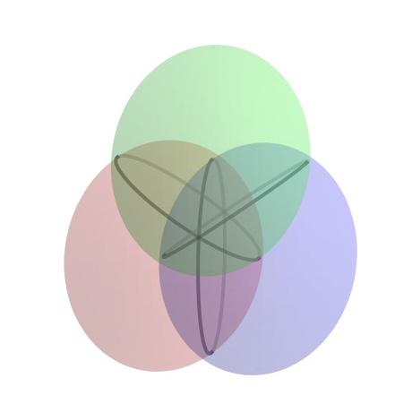
If all measurements were accurate, your position would be at the intersection of the circles centered at $A$ with radius $28$ km, centered at $B$ with radius $26$ km, and centered at $C$ with radius $14$ km as shown in Figure 30.12. Even though the figure might seem to imply it, because of the error in the measurements the three circles do not intersect in one point. So instead, we want to find the best estimate of a point of intersection that we can. The system of equations (30.11), (30.12), and (30.13) is non-linear and can be difficult to solve, if it even has a solution. To approximate a solution, we can linearize the system. To do this, show that if we subtract corresponding sides of equation (30.11) from (30.12) and expand both sides, we can obtain the linear equation

37 x + 7 y + 2 z = 712

in the unknowns $x,$ $y,$ and $z .$

🔗

(c)

Repeat the process in part (b), subtracting (30.11) from (30.13) and show that we can obtain the linear equation

17 x + 37 y + 14 z = 1032

in $x,$ $y,$ and $z .$

🔗

(d)

We have reduced our system of three non-linear equations to the system

\begin{aligned} 37 x & + & 7 y & + & 2 z & = & 712 \\ 17 x & + & 37 y & + & 14 z & = & 1032 \end{aligned}

of two linear equations in the unknowns $x,$ $y,$ and $z .$ Use technology to find a pseudoinverse of the coefficient matrix of this system. Use the pseudoinverse to find the least squares solution to this system. Does your solution correspond to an approximate point of intersection of the three circles?

🔗

Project Activity 30.11 provides the basic idea behind GPS. Suppose you receive a signal from a GPS satellite. The transmission from satellite

i

provides four pieces of information — a location

(x_{i}, y_{i}, z_{i})

and a time stamp

t_{i}

according to the satellite's atomic clock. The time stamp allows the calculation of the distance between you and the

i

th satellite. The transmission travel time is calculated by subtracting the current time on the GPS receiver from the satellite's time stamp. Distance is then found by multiplying the transmission travel time by the rate, which is the speed of light

c = 299792.458

km/s.⁵⁵ So distance is found as

c (t_{i} - d),

where

d

is the time at the receiver. This signal places your location within in a sphere of that radius from the center of the satellite. If you receive a signal at the same time from two satellites, then your position is at the intersection of two spheres. As can be seen at left in Figure 30.13, that intersection is a circle. So your position has been narrowed quite a bit. Now if you receive simultaneous signals from three spheres, your position is narrowed to the intersection of three spheres, or two points as shown at right in Figure 30.13. So if we could receive perfect information from three satellites, then your location would be exactly determined.

🔗
Figure 30.13. Intersections of spheres.

🔗

There is a problem with the above analysis — calculating the distances. These distances are determined by the time it takes for the signal to travel from the satellite to the GPS receiver. The times are measured by the clocks in the satellites and the clocks in the receivers. Since the GPS receiver clock is unlikely to be perfectly synchronized with the satellite clock, the distance calculations are not perfect. In addition, the rate at which the signal travels can change as the signal moves through the ionosphere and the troposphere. As a result, the calculated distance measurements are not exact, and are referred to as pseudoranges. In our calculations we need to factor in the error related to the time discrepancy and other factors. We will incorporate these errors into our measure of

d

and treat

d

as an unknown. (Of course, this is all more complicated that is presented here, but this provides the general idea.)

🔗

To ensure accuracy, the GPS uses signals from four satellites. Assume a satellite is positioned at point

(x_{1}, y_{1}, z_{1})

at a distance

d_{1}

from the GPS receiver located at point

(x, y, z) .

The distance can also be measured in two ways: as

\sqrt{(x - x_{1})^{2} + (y - y_{1})^{2} + (z - z_{1})^{2}} .

🔗

and as

c (t_{1} - d) .

c (t_{1} - d) = \sqrt{(x - x_{1})^{2} + (y - y_{1})^{2} + (z - z_{1})^{2}} .

🔗

Again, we are treating

d

as an unknown, so this equation has the four unknowns

x,

y,

z,

and

d .

Using signals from four satellites produces the system of equations

\begin{aligned} (30.14) & \sqrt{(x - x_{1})^{2} + (y - y_{1})^{2} + (z - z_{1})^{2}} & = c (t_{1} - d) \\ (30.15) & \sqrt{(x - x_{2})^{2} + (y - y_{2})^{2} + (z - z_{2})^{2}} & = c (t_{2} - d) \\ (30.16) & \sqrt{(x - x_{3})^{2} + (y - y_{3})^{2} + (z - z_{3})^{2}} & = c (t_{3} - d) \\ (30.17) & \sqrt{(x - x_{4})^{2} + (y - y_{4})^{2} + (z - z_{4})^{2}} & = c (t_{4} - d) . \end{aligned}

🔗

Project Activity 30.12.

The system of equations (30.14), (30.15), (30.16), and (30.17) is a non-linear system and is difficult to solve, if it even has a solution. We want a method that will provide at least an approximate solution as well as apply if we use more than four satellites. We choose a reference node (say $(x_{1}, y_{1}, z_{1})$ ) and make calculations relative to that node as we did in Project Activity 30.11.

🔗

(a)

First square both sides of the equations (30.14), (30.15), (30.16), and (30.17) to remove the roots. Then subtract corresponding sides of the new first equation (involving $(x_{1}, y_{1}, z_{1})$ ) from the new second equation (involving $(x_{2}, y_{2}, z_{2})$ ) to show that we can obtain the linear equation

2 (x_{2} - x_{1}) x + 2 (y_{2} - y_{1}) y + 2 (z_{2} - z_{1}) z + 2 c^{2} (t_{1} - t_{2}) d = c^{2} (t_{1}^{2} - t_{2}^{2}) - h_{1} + h_{2},

where $h_{i} = x_{i}^{2} + y_{i}^{2} + z_{i}^{2} .$ (Note that the unknowns are $x,$ $y,$ $z,$ and $d$ — all other quantities are known.)

🔗

(b)

Use the result of part (a) to write a linear system that can be obtained by subtracting the first equation from the third and fourth equations as well.

🔗

(c)

The linearizations from part (b) determine a system $A x = b$ of linear equations. Identify $A,$ $x,$ and $b .$ Then explain how we can approximate a best solution to this system in the least squares sense.

🔗

We conclude this project with a final note. At times a GPS receiver may only be able to receive signals from three satellites. In these situations, the receiver can substitute the surface of the Earth as a fourth sphere and continue the computation.

For example, as stated in http://www2.imm.dtu.dk/~pch/Projekter/tsvd.html, “The SVD [singular value decomposition] has also applications in digital signal processing, e.g., as a method for noise reduction. The central idea is to let a matrix

A

represent the noisy signal, compute the SVD, and then discard small singular values of

A .

It can be shown that the small singular values mainly represent the noise, and thus the rank-

k

matrix

A_{k}

represents a filtered signal with less noise.”

Theorem 30.6 is often given as the definition of a pseudoinverse.

statista.com/statistics/203064/national-debt-of-the-united-states-per-capita/

The signals travel in radio waves, which are electromagnetic waves, and travel at the speed of light. Also,

c

is the speed of light in a vacuum, but atmosphere is not too dense so we assume this value of

c